
Instrument Description
Overview of the instrument
From a hardware perspective the instrument partitions into the following key subsystems:
- Pickoff subsystem
- IFU subsystem
- Spectrograph subsystem
- Detector subsystem
- Infrastructure subsystems and electronics
The opto-mechanical parts of the instrument are all contained within a cryostat, operated at a temperature of 120K, while the electronics are on the Nasmyth platform and inside the cable rotator (CACOR; see Figure below).
KMOS has been designed to have effectively three independent modules, each of them comprising 8 pick-off systems, a set of 8 Integral Field Units (IFUs), one spectrograph and one 2kx2k HgCdTe near-IR detector. This ensures that in case of failure of one system, 2/3 of the functionality will still remain. The following section describes the different sub-systems of KMOS in the order they are encountered along the optical path going from the telescope to the detector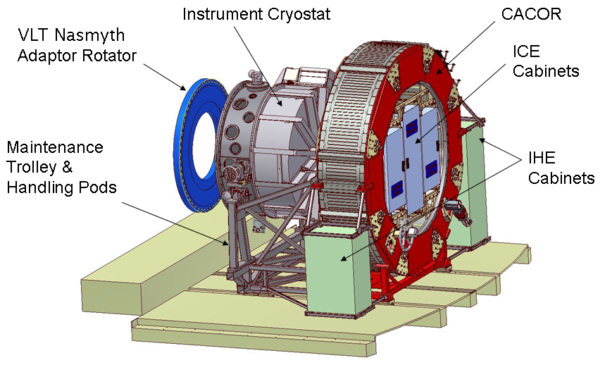
Description of the instrument sub-systems
The pick-off system
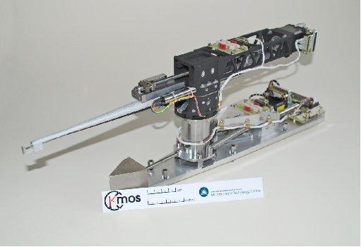
The selection of the pick-off fields is achieved by means of 24 rotating telescopic pick-off arms, which patrol the instrument focal plane of 7.2 arcmin diameter. Each pick-off arm contains a pick-off mirror and associated relay optics, which are positioned inside the telecentric instrument focal plane by means of an articulated arm. The pick-off arms are arranged into two different planes (“top” and “bottom”) of twelve arms each, so that adjacent arms cannot interfere with each other. One of the planes is placed above the nominal focal plane and one below. Each layer of twelve pick-off arms can patrol 100% of the field. The two motions (radius and theta) of the pick-off arms are both driven by stepping motors, which are modified for cryogenic operation. Whilst the positioning of the arms is open-loop via step-counting from datum switches, there is a linear variable differential transformer (LVDT) encoder on each arm which is used to check for successful movement. In addition a hardware collision-detection system is also implemented as a third level of protection which can sense if any two arms have come into contact and stop the movement of arms within 10 µm. All 24 arms can be commanded to move simultaneously and a typical arm movement takes 120 seconds.
 |
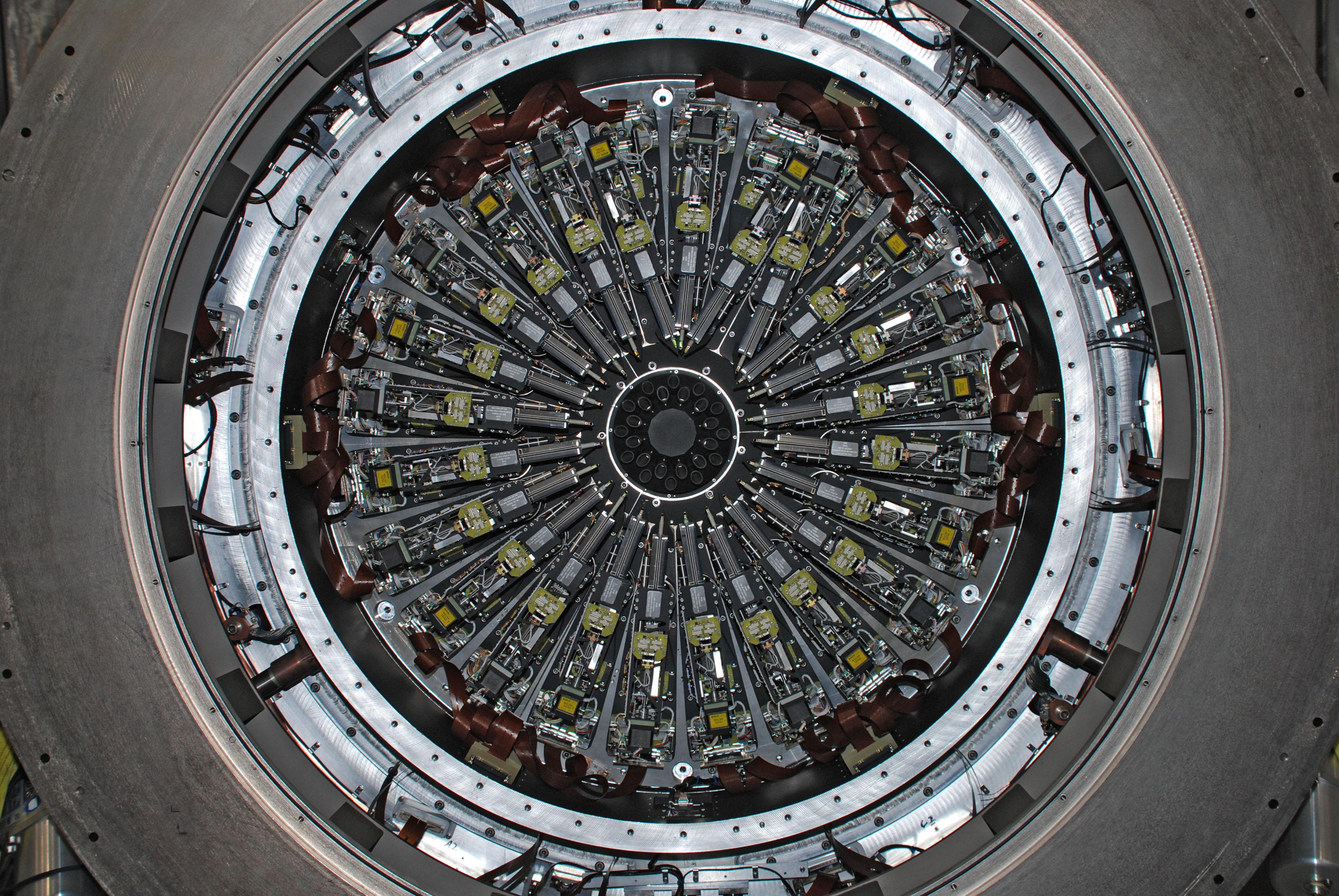 |
Figure 2 Top: one of the pick-off arms; Bottom: the full 24 pick-off arms in the front end of the KMOS cryostat.
Integral Field Units and filters
The IFUs contain the optics that collect the output beam from each of the 24 pick-offs and reimage it with appropriate anamorphic magnification on the image slicers. All the slices from a group of 8 sub-fields are aligned and reformatted into a single slit for each of the three spectrographs. The IFU sub-system has no moving parts and has gold-coated surfaces diamond-machined from aluminium for optical performance in the near-infrared and at cryogenic temperatures.
Each pick-off arm contains a fold mirror located at the tip of the arm to divert the input beam along the arm. A lens is used to collimate the beam and re-image the telescope pupil onto the cold stop located in the arm. A roof mirror which moves in a direction opposite to the fold mirror maintains the optical path length to the cold stop. A subsequent fold mirror then directs the beam along the arm's rotational axis and away from the telescope and towards the K-mirror assemblies. These are used to focus the pick-off fields onto the intermediate focal plane and also to orient each of the 24 fields correctly onto the IFU's image slicer. A set of band pass filters is used to select the appropriate waveband for each observation. As the filters are located in the converging beam produced by the K-mirrors, they are also utilised to correct the chromatic aberrations (focus) induced by the collimating lens in the arm.
Spectrographs
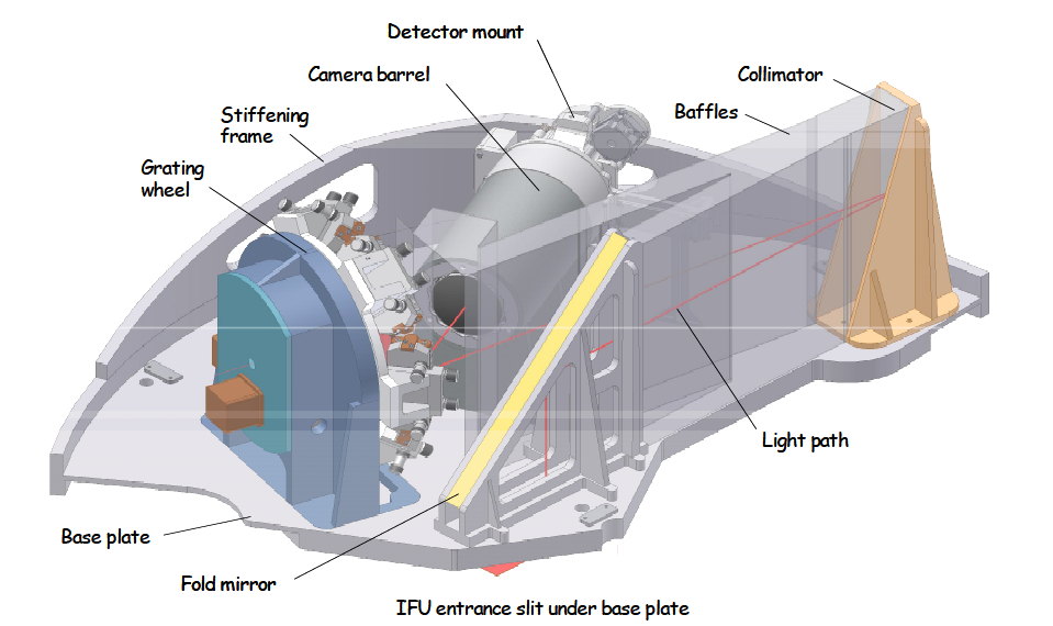
The spectrograph sub-system is comprised of three identical units, which supply three detectors sub-systems. Each spectrograph uses a single off-axis toroidal mirror to collimate the incoming light, which is then dispersed via a reflection grating and refocused using a 6-element transmitting camera. The five available gratings (IZ, YJ, H, K , H+K) are mounted on a 5-position wheel which allows optimized gratings to be used for the individual bands. A 'blank' position is also available for calibrations.
 |
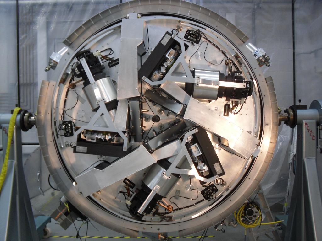 |
Figure 3 Top: Perspective view of a single KMOS spectrograph module. Bottom: the three spectrographs mounted in the KMOS cryostat.
Detectors
KMOS uses 3 Teledyne substrate-removed HgCdTe, 2kx2k, 18µm pixel Hawaii 2RG detectors, one for each spectrograph. The detectors are operated at a temperature of 40K, while the rest of the cryostat is at 120K. Typical characteristics and performances are given in following Table.
|
|
Detector type |
Substrate removed Hawaii 2RG |
Operating temperature |
35K |
QE |
>90% |
Number of pixels |
2048 x 2048 |
Pixel size |
18 m |
Gain (e-/ADU) |
2.08 |
Readout noise (e- ) |
9 for short DIT 2.6 for long integration with Fowler sampling |
Saturation (ADU) |
>60,000 ADU |
Non-linearity |
> 55,000 ADU |
Hot pixels |
~1% |
Minimum DIT (s) |
2.47 |
Sample-up-the-ramp (non-destructive) readout is always used. This means that during integration, the detector is continuously read out without resetting it and counts in each pixel are computed by fitting the slope of the signal vs. time. In addition, Threshold Limited Integration (TLI) mode is used to extend the dynamical range for long exposure times: if one pixel is illuminated by a bright source and reaches an absolute value above a certain threshold (close to detector saturation), only detector readouts before the threshold is reached are used to compute the slope and the counts written in the FITS image for this pixel are extrapolated to the entire exposure time. This is an effective way to remove cosmic rays on these devices (see Finger et al. 2008, Proc. SPIE, Vol. 7021 for a more detailed description).
Important Warning: adjacent pixels can follow different regimes by using this readout mode, one can follow the normal regime and its neighbour can follow and extrapolated regime (if the counts reach the extrapolation threshold). This may lead to bad line profiles, which could then affect chemical abundances determinations, for example. Therefore we strongly recommend to do as short as possible DITs so that the typical counts never reaches 114000e- (or 55000 ADUs) in the ETC (meaning that the count will not be extrapolated).
Calibration unit
The internal Calibration Unit is located inside the cryostat and provides a quasi-uniform light distribution simultaneously to all 24 fields via an 180 mm diameter integrating sphere having 24 output apertures or ports. These ports are divided into sets of 12 (corresponding to the upper and lower arms) and the light from a specific port is directed toward its corresponding pick-off field via one of 24 calibration mirrors located above the focal plane and just outside the patrol field. All calibration sources, tungsten lamp for flat fielding and spectral lamps (argon and neon) for wavelength calibration, are located inside a second external integrating sphere, connected to the internal sphere via a gold-coated light-pipe.
Overall performances
Image quality
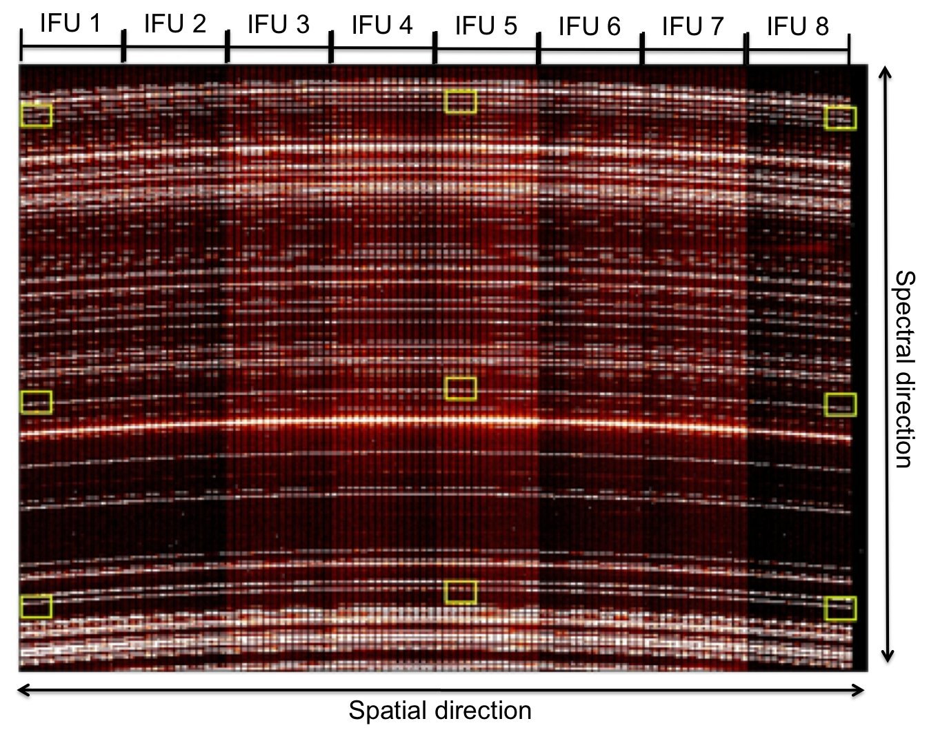
Figure 8 shows one full detector illuminated with arc calibration lamp (argon and neon) in the H-band. Each detector collects the light from 8 IFUs, marked at the top of the image. As in the traditional long slit spectrographs, the spectrum across the array is curved by design, however, this slit curvature is relatively straightforward to correct in software and it is done as part of the data reduction pipeline.
As shown in the zoom-in image in the right panel of Figure 8, the image quality in both spectral and spatial directions is good across the entire array.
The measured FWHM of the spectral lines is 2 pixels, providing a good Nyquist sampling. In the spatial direction, the image of an unresolved point source, shows a FWHM of < 1 pixel (0.2 arcsec) in the direction across the slices and 1.3 pixels (0.25 arcsec) in the spatial direction within the slices.
 |
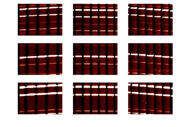 |
Figure 4 Left: One full detector showing the light from the arc calibration lamp (argon + neon) in the H-band. The location of the edges of the 8 IFU imaged onto the detector is shown at the top of the image. The yellow squares on the image mark 9 positions for which a zoom in is provided in the right panel.
Spectral bands
KMOS allows observations across five bands, mostly corresponding to the atmospheric windows in the near-infrared. The wavelength coverage for each of these bands guaranteed in all three is reported in the following table:
Spectral coverage guaranteed in all three detectors.
Band |
Wavelength Coverage (µm) |
|
|
IZ |
0.779 - 1.079 |
YJ |
1.025 - 1.344 |
H |
1.456 - 1.846 |
K |
1.934 - 2.460 |
HK |
1.484 - 2.442 |
Due to the spectral curvature, not all the IFUs have the same wavelength coverage. The IFUs imaged at the centre of the array have a slightly different wavelength coverage compared to the IFUs at the edge of the array. For completeness the wavelength coverage for IFUs at the at the centre and edge of the array, for all three detectors are reported in the following Table:
Spectral Coverage at the centre of the detector
Band |
Wavelength Coverage (µm) |
||
|---|---|---|---|
|
Spectrograph A |
Spectrograph B |
Spectrograph C |
IZ |
0.778 - 1.092 |
0.779 - 1.094 |
0.771 - 1.085 |
YJ |
1.022 - 1.359 |
1.025 - 1.361 |
1.015 - 1.352 |
H |
1.452 - 1.866 |
1.456 - 1.870 |
1.443 - 1.857 |
K |
1.921 - 2.460 |
1.922 - 2.461 |
1.919 - 2.460 |
HK |
1.474 - 2.471 |
1.484 - 2.481 |
1.458 - 2.456 |
Spectral Coverage at the edge of the detector
Band |
Wavelength Coverage (µm) |
||
|---|---|---|---|
|
Spectrograph A |
Spectrograph B |
Spectrograph C |
IZ |
0.772 - 1.086 |
0.773 - 1.087 |
0.764 - 1.079 |
YJ |
1.014 - 1.351 |
1.016 - 1.353 |
1.007 - 1.344 |
H |
1.441 - 1.855 |
1.445 - 1.859 |
1.432 - 1.846 |
K |
1.932 - 2.472 |
1.934 - 2.473 |
1.931 - 2.472 |
HK |
1.465 - 2.462 |
1.470 - 2.442 |
1.445 - 2.442 |
Spectral resolving power
The measured spectral resolving power in all 5 bands is shown in the following Table:
Band |
Pixel scale nm/pixel |
Resolving power Short wavelength |
Resolving power Band centre |
Resolving power Long wavelength |
|---|---|---|---|---|
IZ |
0.143 |
2795 |
3406 |
3773 |
YJ |
0.165 |
3089 |
3582 |
4088 |
H |
0.203 |
3570 |
4045 |
4555 |
K |
0.266 |
3809 |
4227 |
4883 |
HK |
0.489 |
1514 |
1985 |
2538 |
Sensitivity
The total efficiency of KMOS in all bands has been measured on sky using several standard stars observed during commissioning. Based on these values the expected limiting AB magnitudes in 1 hour on-source observation for S/N of 5 per spectral bin are given in the following table:
Band |
Magnitude (Vega) |
|---|---|
| IZ | 19.9 |
| YJ | 20.1 |
| H | 19.8 |
| HK | 19.8 |
| K | 17.9 |
For short exposures the minimum DIT is 2.47s and to reduce the calibration load and share calibrations with other projects we recommend especially in service mode the following DIT values: 2.47s, 3s, 4s, 5s, 10s, 15s, 20s, 30s, 60s or 100s.
For long exposures on faint targets with no risk of saturation we recommend to work with NDIT=1 and a DIT depending on the frequency of sky frames needed. To avoid excessive daytime calibrations, only a limited choice of DIT values for longer exposures is recommended in service mode: DIT = 300s, 400s, 480s, 600s, 900s, 1200s.
It is worth noticing that background limited performances are reached for exposures times >= 300s
The Exposure Time Calculator
The KMOS Exposure Time Calculator (ETC) can be found at the following link:
http://www.eso.org/observing/etc/
It returns a realistic estimation of the integration time (on source!) needed to achieve a given S/N as a function of the band and selected and the atmospheric conditions. In building the OB please remember to add the overheads for time spent on sky and telescope/instrument setting as described in section 3.5.
The parameters to be provided for the input are standards and self-explanatory. The magnitudes for the targets can be specified for a point source or for an extended source. Results can be given as exposure time on source needed to reach a given S/N or as the S/N reached in a given exposure time on source.
In the screen output from the ETC the S/N is given per spectral pixel, not per resolution element. Therefore to compute the S/N per resolution element it is necessary to sum over 2 pixels.