The last line above means that all other files except the wavelength map will be the defaults (i.e. run the tool with parameter -d).

Clean-up

Note that when using the tool stand-alone, the user has to take care of cleaning the results directory every now and then, e.g.:

rm -rf /tmp/reflex_tmp_forsSpecTool-*

Examples

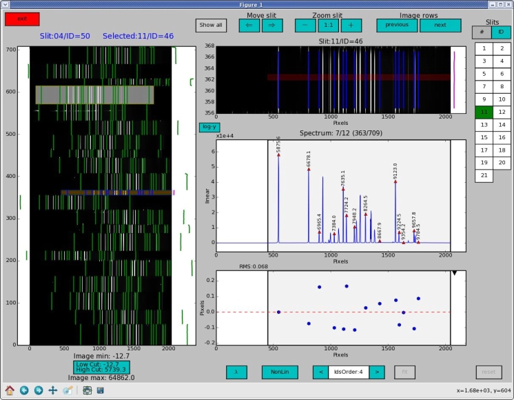
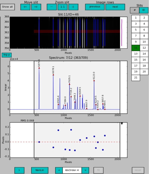
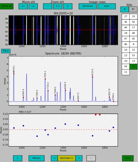
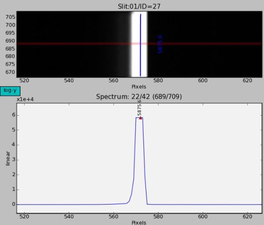
The first example screenshot below is right after start-up. The example in the picture below is for the seventh row in the eleventh slit. In this example there are 21 slits containing 709 rows in total.

Below are explained all the buttons of the tool.

for exiting the tool.

return all windows to original mode in current slit and image row.

for toggling between linear and logarithmic scale in rectified/reduced lamp spectrum profile window (middle right side).

for moving/zooming the three right side windows in horizontal direction.
See below note for matplotlib pan/zoom mode.

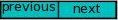for moving to preceding and subsequent image row.

for toggling between displaying slit number or slit ID in the slit buttons, current mode is painted gray.

• slit buttons are displayed in two columns, clicking a button will display the center image row of the chosen slit, current slit is green.

for returning to initial values.

for refitting the current slit with new polynomial fitting order (IdsOrder) and/or deleted/recovered lines.

for decreasing/increasing the wavelength calibration polynomial order, valid range is 2-5.

for toggling between different images (residuals of fit, non-linear part of fit, pixel versus wavelength) in the fit results window (lower right side), the next available mode is printed on the button.

for toggling X-axis between pixels and wavelengths in the three right side windows, the two upper windows (single slit and spectrum profile window) are toggled between RECTIFIED_LAMP_MXU (X-axis in pixels) and REDUCED_LAMP_MXU (X-axis in &lambda), the next available mode is printed on the button.

for changing the cuts of the images in the all slits and single slit windows.

Line identification window (all slits)

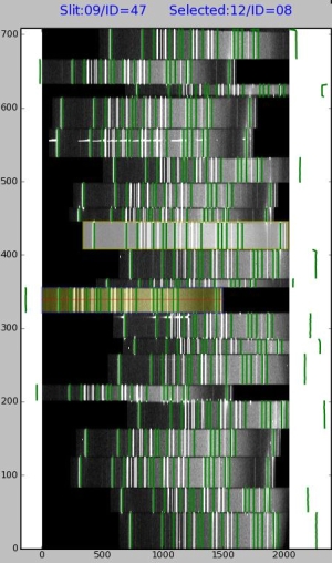
Window image shows the slit locations and spectrum with identified lines which are plotted over the spectrum. The lines illuminate the grade of quality with current line catalogue and inverse dispersion solution polynomial fitting order. The goal is to find anomalies in identified line locations.

Usage

Slit number and slit identification number are shown on top of the image window. Left side shows the slit upon which the cursor is currently and right side is the selected (activated by clicking) slit.

Mouse options

When moving mouse over image the slit under mouse pointer will be highlighted and surrounded by a yellow box.
The slit can be selected by clicking the left mouse button. Selected slit will be highlighted yellow.
Current image row is shown with a red bar over the current slit.

Toolbar

The matplotlib default toolbar has options which are useful for the image zooming and panning.

The home button will return the image as it was in launch. A known problem is that in this tool this does not always work properly (e.g. when spectrum profile window is in logarithmic scale).

Left and right arrows will work as a 'undo' and 'redo' when zooming or panning image.

Pan with left mouse, zoom with right. NOTE: matplotlib pan/zoom mode must be applied to the single slit window, and when mouse button is released the changes done will reflect to the two windows below it keeping the X-axis scale identical in all the three right side windows. Note that the script blocks moving/zooming the single slit window in vertical direction.

Zoom area to rectangle.

Spectra of one slit, spectrum profile and results of fitting

The right-hand side of the tool window has three windows.
When X-axis is in pixels, active area of slit is painted light gray in the two lower windows.

Single slit spectrum

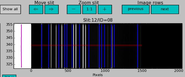
The upper window plots the current single slit (highlighted in the left-side window).

Current image row is shown with a red bar. Image row can be chosen by clicking on single slit window, but NOT in matplotlib pan/zoom mode.

The dispersion solutions for the identified lines calculated with the wavelength calibration polynomial coefficients are shown with blue lines.

For zoom/move buttons see above where all the buttons are explained.

When X-axis is in pixels, the single slit and spectrum profile windows contain the RECTIFIED_LAMP_MXU (produced by fors_extract_slits) versus X CCD position of the current image row.

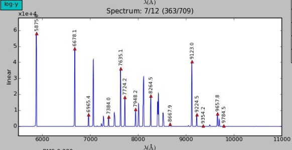
When X-axis is wavelengths, the single slit and spectrum profile windows contain the REDUCED_LAMP_MXU (produced by fors_wave_calib) versus wavelength.

Spectrum profile

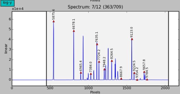
The middle window shows the spectrum profile of one image row. The current image row is printed above the window: the current slit contains 12 rows and all the slits together contain 709 rows.

The peak positions of the spectrum are marked with red triangles. The identified line wavelength is printed above the peak.

Results of fitting

The lower window plots at start-up the residuals of the fit versus X CCD position for the current image row.

Lines outside active area or not found by the fitting are indicated with a black triangle down in the upper edge of window.

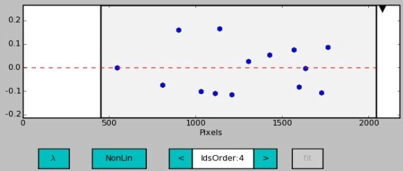
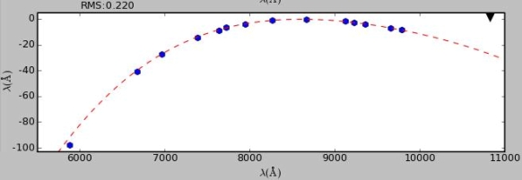
In addition to residuals the non-linear part of the fitting and pixel position can be plotted (second button from the left below window).

The X-axis can be toggled between pixels and wavelength (first button from the left below window).

Deleting of line(s)

Click with left mouse button blue ball(s) in the lower window. The ball will turn red and activate the fit-button. You can cancel your intended deletion with right mouse button. The refit is done by pressing the button. After refitting, a red triangle down in the upper edge of the fit results window will indicate the line(s) deleted by the user.

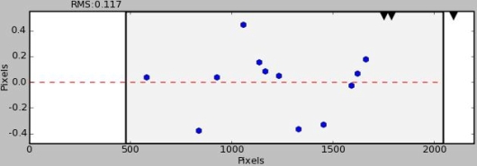
In the figure below two lines with clearly larger residuals are marked for deletion and the fit button is active. In the slit columns are shown the slit IDs.

In the figure below the refitting has been done and the positions of the two deleted lines are marked with a red triangle down in the upper edge of the fit results window. The RMS improved from 0.071 to 0.027. Consider however also this point: the more lines, the better indicator the RMS is, and the more stable the solution.

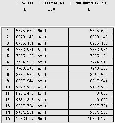
The tool produces a fits table that keeps track of the lines deleted by the user. The first two columns are a copy of the original line catalog. When a line is removed from a slit, a new column with the removed line(s) set to zero is added.

Recovering deleted line(s)

Deleted lines can be recovered by clicking with left mouse button the red triangle down turning it blue. You can cancel your intended recovering with right mouse button. The refit is done by pressing the button.

In the figure below the other one of the two lines deleted in the previous step is marked for recovery and the fit button is active.

Changing the polynomial order of the fitting

Click either arrow beside the IdsOrder box to decrease/increase the polynomial order. This will activate (turn green) the fit button. The refit is done by pressing the button after which the polynomial order of the current slit is stored to the new value. If you move to another image row before pressing the fit-button the polynomial order will be restored to the original value and the fit-button deactivated.

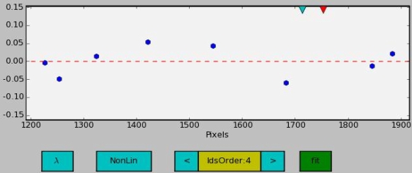
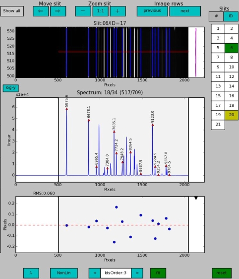
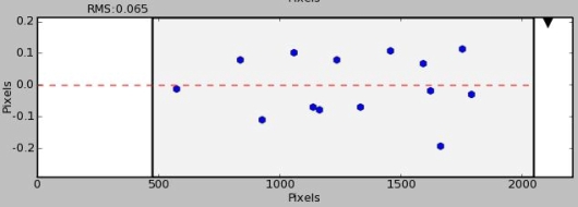
In the figure below we first of all see that the slit button number 20 is yellow because this slit was changed in the previous step. Secondly the reset button is active (green) since we have made changes. Now we decrease the polynomial fitting order of the current (slit button number 6 is green) slit and refit it. The tool runs the recipe fors_wave_calib with parameter --wdegree set to IdsOrder.

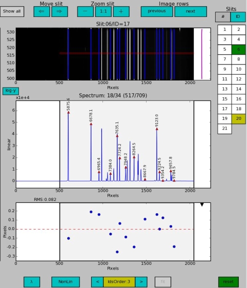
In the figure below we see that the previous step was not a good idea since RMS worsened from 0.06 to 0.082.

In the fits table disp_coeff_mxu_new.fits produced by the tool (that reruns fors_wave_calib), you will see that column c4 of the rows 500-533 has changed to zero. These rows correspond slit number 6 for which we changed the fitting order from 4 to 3. Increasing the order to 5 would create column c5.

Example of bad fit

In the two figures below is slit number 1 fitted with polynomial order 2. Here we have a much worse (larger residuals, less lines identified) solution, and we see systematic errors.

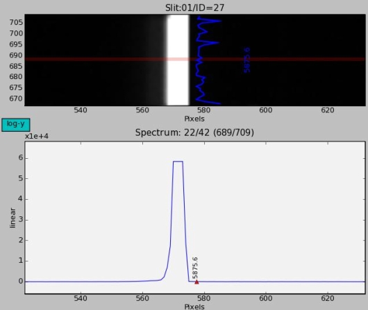
Example of good fit

In the two figures below is slit number 1 fitted with polynomial order 4. The solution is much better than above, and introduces random errors.

Notes

The refit is in both cases (deleting/recovering lines and changing fit order) done for one slit at a time. A refitted slit is indicated by painting yellow the IdsOrder box and the slit button. After the first refit the reset button is activated (turned green).

The combined number of blue/red balls and black/red/blue triangles down in the fit results window equals always the number of lines in the original line catalog.

In the fit results window red/blue balls and black triangles down are per image row, red/blue triangles down are per slit. Note the difference with the skyline alignment tool.