
DATABASE OF TECHNICAL DATA
PSF FITTING
Introduction
As explained here the PSFs simulated by ESO's numerical end-to-end tool OCTOPUS are computationally very expensive and so they typically only cover a few seconds of real time. As a result these PSFs show residual speckles. In addition, the PSF images are quite large (4k × 4k pixel) and hence they are a bit unwieldy when used for the simulation of astronomical images. Finally, the contrast between the centre and the edge of a PSF image varies from PSF to PSF, depending on wavelength and AO type.
To overcome all of these limitations we have developed a software tool called eltpsffit. This tool allows the user to fit a combination of different analytical functions to a given PSF image. The result is a representation of the PSF that is speckle-free, fully specified by just a few or at most tens of parameters, and which can be extrapolated to arbitrary contrast levels (or rather as far as one is prepared to trust the fit). Here we describe how to install eltpsffit on your computer and how to use it. The code is written in C and it is free software (but please see this).
Obtaining the code
You can obtain the source code for eltpsffit here. The current version is 1.1. See the README file that comes with the distribution for a list of changes from earlier versions.
Compiling and installing the code
Compiling and running eltpsffit requires a number of libraries to be installed on your system: PGPLOT including its C extension cpgplot, CFITSIO, wcssubs (or WCSTools), and GSL. All of these are very commonly used libraries and they are all part of ESO's scisoft collection. Hence they may well be installed on your system already.
After unzipping and unpacking the eltpsffit tarball you will find a
directory called eltpsffit-[version_number]. It contains the README file and a subdirectory src/ in which you'll
find all the source code, header files and a Makefile. Ideally you
only need to type > make in the src/ subdirectory to
compile the code and to obtain an executable. However, you may need to
edit the top of the Makefile a bit if there are any problems in
locating the various libraries and/or include files. For example, if
library x cannot be found you may need to add '-L/path/to/library/x/'
before the '-lx' switch. Similarly, if some include file cannot be
found you may want to add the switch '-I/path/to/missing/file/' to the
CFLAGS.
Running the code and performing a fit
The following is intended to be a step-by-step guide on how to use eltpsffit to obtain a fit for a given PSF. We will use the LTAO, K-band, zero zenith distance, on-axis PSF as an example to work on. To follow this guide, download this PSF image and save it off as 'psf.fits'.
To run eltpsffit simply type > eltpsffit
psf.fits Running eltpsffit without any arguments or
with the switch '-help' will produce a short usage message including a
list of command line options which will be discussed later. On
start-up eltpsffit displays an empty black window and asks
whether the user wants to fit a cut along the x-axis of the
PSF. Possible replies are 'n' for no and 'y' for yes (or simply hit
'return' to accept the offered default). Fitting a cut of the PSF may
be useful under some circumstances but we will skip this step here, so
answer 'n'. Same for the next question about fitting a cut along the
y-axis. The third question is whether you would like to fit the PSF's
radial profile. Answer 'y'. eltpsffit will now compute the
flux centroid of the image and the spherically averaged flux profile
around the centroid in annuli of 1 pixel width. This computation may
take several minutes, so be a little patient. Once completed
eltpsffit will display the profile on a log scale versus the
distance from the centroid in milliarcsec in the formerly empty black
window. The window will also change its size. Unfortunately, it cannot
be resized by dragging the window frame. If it is too large for your
screen (e.g. when working on a laptop) do the following: type 'Ctrl-q'
in the plotting window (not in the terminal from which you started
eltpsffit), answer the subsequent question in the terminal
with 'n' (this will be discussed later), and then restart
eltpsffit using the '-ws' switch. For example,
eltpsffit -ws 17 psf.fits works well for a laptop
screen. Return to the current point by answering 'n', 'n' and 'y' to
the three questions as before (just accept all the defaults). Notice
that this time round you did not have to wait for the computation of
the radial profile because eltpsffit saved it on the previous
run. You should now see something like this.
From now on we will interact with eltpsffit by typing single key strokes or clicking the mouse in the plotting window. You can obtain a list of available commands by typing '?' in the plotting window. The first thing you may want to do is to look at the data in more detail, i.e. to navigate around the plot. For example, to examine the core of the PSF hit 'w', then click the left mouse button (lmb) slightly above and to the left of the innermost data point, then drag out a rectangle to cover the region you would like to zoom in on, and click again. Typing 'w' followed by 'a' returns the plot to the original view. You can obtain a list of all available windowing commands by typing 'w' followed by '?'. As one needs to navigate around the plot a lot during the fitting process it is useful to familiarise yourself with these commands. Just try them out. (NB: we have modified the PGPLOT library in order to allow the dragging of the whole plot and the use of the mouse's scroll wheel to zoom in and out just like on a google map. This makes it much easier to navigate.)
We now need to set up a starting point for the fit. Recall that we wish to fit the PSF with a combination of one or more analytical functions, i.e. the fitting function is simply the sum of a number of components. We now need to choose these components and determine suitable 'first guesses' for their parameters. This is done by adding in components one by one and by interactively adjusting their parameters until we get a reasonable starting point. Each component may be chosen to have one following funtional forms:
- Gaussian
- Lorantzian
- Moffat function
- Sinc function
- Airy disk
- Obstructed Airy disk
- Constant
Once you have adjusted the parameters to your satisfaction zoom out again. You will notice that the obstructed airy disk component does not extend to large radii but is truncated. This truncation occurs only for components of type 'airy disk' or 'obstructed airy disk' but not for any of the other types. It prevents the occurrence of small wiggles at large radii which was emprically found to improve the achievable quality of the final fit. The truncation radius is a fixed multiple of the component's width and this parameter is hardwired into the code. If you wish to change it, you need to edit the parameter AIRC in the file eltpsffit.h in the distribution's src/ directory, and recompile the code.
Let us now add a second component to our model to represent the seeing halo of the PSF. Zoom out to full view, hit 'a' and select the component type 'mx' (Moffat function). Appending the letter 'x' to the component type's designation will tie the position of the component to that of another, already existing component. In our case there is only one other component (the obstructed airy disk) and so the second component's position is tied to that of the first. If it is not obvious which existing component the new component should be tied to you will be asked to identify one by its index (i.e. '1' for the first component, '2' for the second, etc.). It is also possible to fix a parameter at its current value, meaning that this parameter will not be adjusted during the fit. This is achieved by hitting 'x' on the parameter's handle. Hit 'x' again to release the parameter again. For example, it is a good idea to fix the position of the first component at a value of 0 mas (zoom in on the centre, adjust the position of the first component to be very close to 0, hit 'x' on the handle, and answer the resulting question with 'p' for position). Note that fixing the position of a component to which other components' positions are tied fixes all of them.
Once you have adjusted the parameters of the second component to your satisfaction you should have something like this. This might be a good time to save the work you have done so far by hitting 'Ctrl-s'. If you quit and restart eltpsffit now the code will automatically find and read in the saved model so that you can continue working where you left off. 'Ctrl-s' also writes out the profile of your current model which may be used by external applications or just to examine your model. Also try hitting 's' now which shows you the current model in the terminal window: one line for each component, listing the component's type, height, position, width, and a fourth parameter which corresponds to the obstruction parameter and Moffat index for the first and second components, respectively. (For any other component type this parameter would be 0.) Each parameter is followed by an integer which indicates whether the parameter is fixed (0) or not (1). The position parameter is also followed by an integer which gives the index of the component to which this component's position is tied (0-indexed).
Hitting 's' also shows you the fit statistics. These are pretty meaningless right now, as we have not yet performed a fit. However, this also caused eltpsffit to calculate the residuals of the current model which you can now examine by typing 'r'. The horizontal orange lines represent the (arbitrarily chosen) 'target': it is usually possible to obtain a fit that lies within 5% of the data almost everywhere, except for some larger deviations on small scales (which unfortunately usually includes the core). Typing 'r' again toggles back to the PSF. Note that you can also toggle between the current log scale and a linear scale by typing 'l'.
Before we can perform our first actual fit we must decide how to weight the individual data points in the fit. Usually the weights would be the inverse variance of the data but the simulated PSF data do not have any errors attached to them. Essentially, we are free to choose the weights to achieve what we want. For example, if we give each data point the same weight the fit will try to make the residuals roughly equal everywhere on a linear scale. Since both the data and all of the different fitting functions are close to 0 at large radii the fitting procedure will concentrate on getting the fit 'right' in the centre. In contrast, if we set the weight of a data point to be proportional to the data value (meaning that the weights are all equal in log space) then the fit will try to make the residuals roughly equal everywhere on a log scale, giving relatively more weight to the points at larger radii. Because it is not a priori obvious what the goal of the PSF fitting should be (presumably it will depend on the ultimate application) eltpsffit allows you to choose among the two options discussed above as well as a third, intermediate option where the weight of a data point is proportional to the square-root of the data value.
Setting the weights is done by hitting 'z' to enter a special weight setting mode (hit '?' now to obtain a list of available commands in this mode) and then either '1', '2' or '3' to select one of the above schemes. However, before we can do this we need to set an appropriate proportionality constant in order to get a reasonable overall scale for the weights. For historical reasons this is currently done in a somewhat awkward, complicated way. In a future version eltpsffit will determine this automatically but for now you will just have to bear with us and just follow these instructions: make sure you are in normal mode. If you are still in the special weight setting mode then leave it by hitting 'q'. When in normal mode, plot the residuals on a log scale (use the 'r' and 'l' keys). Zoom in a bit on the y=0 axis until you have something similar to this. Now enter the weight setting mode again by typing 'z'. Now hit 'f'. You should see something like this. The orange line shows the result of sliding a boxcar (of width 51 pixel) along the residuals and calculating the rms of the residuals within the boxcar at each point. The rms of the residuals seems to fall off linearly with radius, except for some large excursions from this trend ar r < 800 mas, near r = 1800 mas, and near r = 2700 mas. The green line shows a linear fit to the orange line. Obviously, it doesn't capture the trend because the fit was thrown off by the large excursions. We will now exclude these regions from the fit: place the cursor at some r < 0 and hit 'k'. Move the cursor to r = 800 mas and hit 'k' again. Hit 'f' again and you should now see this. The points we just excluded are now marked by small crosses, and the green line now comes close to representing the underlying trend of the rms residuals. Repeat the exclusion process and fitting as above for the remaining two regions of large rms values until you arrive at something like this. We are now finally ready to set the weights by hitting '1', '2' or '3'. Here we will choose option '3', which also leaves the weight setting mode, returning you to normal mode. You can now make the weights visible as error bars by hitting 'e' (hit 'e' again to turn them off again).
The complicated procedure above only ever needs to be done once for a given PSF. If you now want to change from constant log weights to constant linear weights just type 'z' and then '1'. Type 'z' and '3' to go back to constant log weights. Now type 'Ctrl-s' which will save not only the current model but also the weights you have just defined so that they will be available again if you quit and restart eltpsffit on the same PSF.
Now that the weights are defined we can venture a first fit. Go to the full view of the data in log space and hit 'F' (note the capital letter). In the terminal you will see the progress of the fit at each iteration, with the final model parameters and fit statistics being displayed once the fit is completed. Note that the chi^2 values are pretty meaningless, since our weights do not really represent errors. They are only useful for comparing two different models. The new fit is also displayed in the plotting window. Hit 'c' to turn off the plotting of individual components (hit 'c' again to turn it on again) and you should see something like this with residuals looking like this.
You can now continue to improve the fit. In order to achieve a fit that meets your requirements you have the following tools at your disposal: adding more components, fixing component parameters, and choosing different weighting schemes. In addition you may also reject some data points from the fit: just hit 'k' at either end of the range that you want to reject. These data points will now be marked by red crosses and will not be used in any future fits. As you work to improve the fit, remember to hit 'Ctrl-s' once in a while to save your work. If a fit has screwed up your model for some reason you can return to a previously saved version by typing 'Ctrl-r'.
Once you are satisfied with your fit, hit 'Ctrl-q' to exit the fitting of the radial profile. On exit, the present model is saved again. In the terminal you will now be asked if you would like to fit a spherically symmetric 2D model to the image, meaning that the spherically averaged profile and the image centroid will be fit simultaneously. Unfortunately, due to memory allocation problems this mode does not yet work properly. However, you can nevertheless answer 'y' to this question. eltpsffit will now attempt to read in a previously saved 2D model. Failing this it will look for a previously saved 1D radial profile model (i.e. the model you have just produced above). Using the previously computed flux centroid of the image this 1D model is then converted to a spherically symmetric 2D model to be used as the starting point for the 2D fit. Similarly, the weights and rejected points of the 1D case are also automatically adapted to the 2D case. Normally, eltpsffit would now launch the fitting process but this step is currently disabled. The code proceeds to write out the best fit 2D model (which is currently identical to the input model), as well as the radial profile of the 2D model (which is currently identical to the radial profile of the 1D model) and an image of the 2D model. Obtaining this image is currently the main reason to go through the 2D 'fitting' process as it allows the user to visually asses the quality of the fit by blinking the original PSF image with this model image. Once everything is written out the whole fitting process is complete and eltpsffit will exit.
To provide an example of what the final result of the fitting process might look like, we have performed detailed fits of two PSFs: the relatively high-Strehl PSF used in the step-by-step guide above (LTAO, K-band, zero zenith distance, on-axis) and a low-Strehl PSF (GLAO, U-band, zero zenith distance, 6 arcmin FoV, on-axis). You can download the PSFs and the files generated by eltpsffit during the fitting process from here and here, respectively. In particular, if you download the .1drf and .1drwr files (see below for the meaning of these files) along with the PSF image, our best-fit model will be automatically read in when eltpsffit is run on that PSF so that you can examine it in detail and modify it if you wish. The two figures below directly compare the images of the above two PSFs with images of our best fit models.
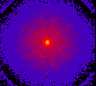 |
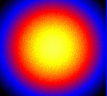 |
| Data/model comparison for a high-Strehl PSF | Data/model comparison for a low-Strehl PSF |
Output files
The process described above results in a number of files that eltpsffit writes to your present working directory. These files have the same root file name as the PSF that you have fit, but with different extensions. Each file contains a header with a brief description of its content.
File
Description
Getting help
If you encounter any problems during the compilation of eltpsffit or have any questions regarding its use please contact Joe Liske.
License / Disclaimer
Copyright (C) 2009 by Jochen Liske.
This program is free software: you can redistribute it and/or modify it under the terms of the GNU General Public License as published by the Free Software Foundation, either version 3 of the License, or (at your option) any later version.
This program is distributed in the hope that it will be useful, but WITHOUT ANY WARRANTY; without even the implied warranty of MERCHANTABILITY or FITNESS FOR A PARTICULAR PURPOSE. See the GNU General Public License for more details.
E-ELT Science
What's New?
- 05 Dec 2014
Spending on first construction phase approved
Science Case
Project Science Team
Phase B (2006 – 2011)
- Science Working Group
- Design Reference Mission
- Design Reference Science Plan
- Tools: Imaging ETC / Spectroscopic ETC / Other software