
MUSE p2 tutorial: WFM-NOAO observations of an extended object
The Phase 2 process begins when you receive an email from ESO telling you that the allocation of time for the coming period has finalized and that you can view the results by logging into the User Portal and clicking on "Check the web letters." Note that the username and password that you need to use for the User Portal are the same as those you will use to prepare your OBs.
You follow the instructions given by ESO and find that time was allocated to your run with MUSE. Therefore, you decide to start preparing your Phase 2 material, which consists of a README file, and one or more OBs equipped with finding charts.
In what follows we will discuss and focus on concepts that are only specific to MUSE observations, therefore assuming you have read the p2 documentation and, as such, you are familiar with the general concepts of p2, and its features.
Goal of the run
In this tutorial we will prepare an OB for a simple example observing run, consisting of IFU observations of the galaxy M64, RA(2000)= 12:56:43.696 , DEC(2000)= 21:40:57.570, by using the WFM-NOAO-N mode. It is intended to provide an example of a mosaic MUSE observations of an extended object, therefore with off-target sky monitoring, but with no particular requirement on the target centring accuracy.
The observing strategy based on the science requirements is:
- WFM-NOAO-N
- VLT Guide Star selection
- Sky monitored off-target (i.e., sky exposure taken few arcmin away from the target)
- Mosaic of ~3'x1' area on target performed with a total of 6 exposures
Getting started
For the sake of this tutorial, we will use the p2 demo facility, which allows users who do not have their own p2 login data to still use p2 and prepare example OBs (for instance during the Phase 1 preparation to get the overheads right!). You cannot use it to prepare actual OBs intended to be executed. When you prepare OBs that should be executed in PARANAL you must use your ESO User Portal credentials to log into the p2 (with http://www.eso.org/p2).
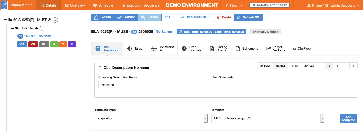
After directing your browser to the p2, and creating an empty new OB under your SM MUSE run ID by clicking on the OB icon, the main p2 GUI will appear as follows (note that the p2 GUI is regularly updated and might look slightly different):
OB general sections
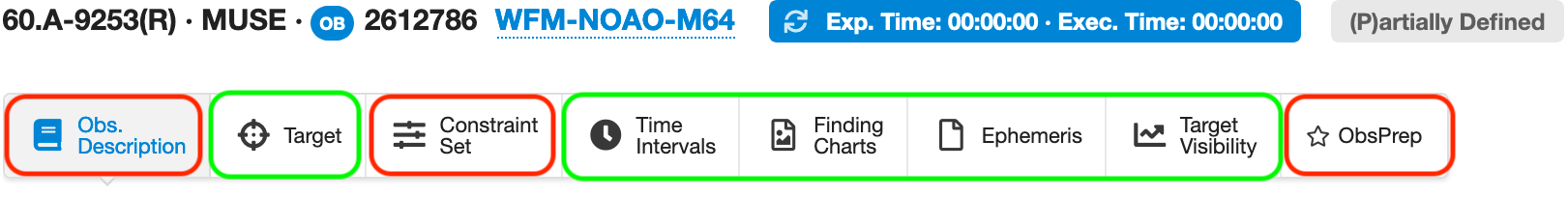
Your newly created OB consists of general (Target, Time Intervals, Finding Charts, Ephemeris, Target Visibility) and instrument specific (Obs. Description, Constraint Set and ObsPrep) sections that in the figure below are highlighted in red and green, respectively. Each section is accessible through the corresponding tab that appears just below the OB name.
Filling the general OB sections should be fairly straightforward (i.e. Target name, RA and DEC etc..) because each field has its own mini help accessible to users when moving the mouse over it. However, should you need more detailed instructions please consult this page.
OB instrument specific sections
1. Constraint Set
By clicking on to the Constraint Set tab you access the corresponding section, where you will have to provide constraints on airmass, Sky Transparency (i.e., Photometric, Clear, Variable thin cirrus, Variable thick cirrus), Lunar Illumination, Image Quality, Moon Angular Distance, Twilight (min) and Precipitable Water Vapor (mm). While defining the OB constraints you should always remember that Phase 2 constraint must agree with Phase 1 request. Details on each specific constraint (i.e., range and meaning) can be found in the general and specific observing conditions pages.

Screenshot of the Constraint Set section. Note that the Turbulence constraint is only applicable for the NFM case. For WFM observations, the relevant parameter describing the seeing is the Image Quality, which refers to the FWHM on a MUSE image at the requested airmass and measuread at 700nm. The Image Quality value is given by the ETC when using Phase 1 constraints as input parameters.
2. Obs. Description: the Acquisition template
The Obs. Description section should be regarded as the core of any given OB because it contains the details of the observations, arranged in templates. Each OB must have an acquisition and one or more science templates.
Selecting the right acquisition template
The instrument mode is defined in the acquisition template, therefore each mode has its own dedicated acquisition template. As summarised in this table, for the case of seeing limited observations with the WFM there are two possible acquisition templates (MUSE_wfm-noao_acq_preset and MUSE_wfm-noao_acq_movetopixel) depending whether or not a precise (within ~0.3") target centring is required.
In this example the target is a very extended object, therefore we assume that a pointing accuracy of few arcsec is sufficient. When no manual interaction (e.g., fine-tuned adjustment of the field) is needed, the MUSE_wfm-noao_acq_preset acquisition template is the best choice because it is the fastest one.
Once you have decided which acquisition template matches your observational needs, click on to the Obs. Description tab to access the corresponding section and select the acquisition template as shown in the picture below. Then click on the "Add Template" button to access the content of the template.

Filling the acquisition template
The set of acquisition parameters appearing on the p2 GUI after loading the MUSE_wfm-noao_acq_preset template can either be defined completely manually or in a more automatic way by using ObsPrep.
In what follows we first provide a short desciption of each parameter, and then we will use ObsPrep to fill in the template.
- Start slow-guiding?: The MUSE derotator produces a residual mechanical wobble, which produces a repeatable pattern as a function of the derotator position. The effect of this wobble can be compensated by the slow-guiding system (SGS) when point-sources are present in the metrology field outside the FoV (i.e., the four banana-shaped areas). Therefore, it is strongly recommended to enable the SGS if i) suitable sources are present in the metrology fields; ii) the target is neither a moving object nor a high proper motions source; and iii) the on-target exposure time is longer than 4 minutes. Four minutes is in fact the minimum interval of time after which offset corrections are sent from the slow guiding system to the telescope.
- Alpha offset for the target (arcsec): RA offset between the target and the reference star to be used for accurate target centring (i.e., optional as it applies only in case the blind-offset procedure is performed, see dedicated note below)
- Delta offset for the target (arcsec): DEC offset between the target and the reference star to be used for accurate target centring (see dedicated note below).
- RA of guide star: RA coordinate of the VLT guide star (VLT-GS, see dedicated note below)
- DEC of guide star: DEC coordinate of the VLT-GS
- Get Guide Star from: If left to CATALOGUE then the VLT-GS is selected by the telescope operator (see note below)
- Position Angle on Sky (deg): Orientation of the MUSE FoV
- Instrument Mode: Select the desired filter (i.e., Nominal or Extended)
Special Note on the VLT-GS:
Suitable VLT-GSs should not be closer than 4' from the MUSE field center but still within the VLT unvignetted FoV (i.e. within 11' radius) and should have a magnitude in the range: 11<R<13.5. The position of the selected VLT-GS is provided by the user in the acquisition template through the star's absolute coordinate (i.e. RA of guide star, DEC of guide star). The parameter Get guide Star from must be set to SETUPFILE in case a specific star is given. Finally, the selection of the VLT-GS is optional, however users are encouraged to define a VLT-GS in the OBs in case the observing strategy requires: i) stacking together multiple OBs (i.e., by selecting for all similar OBs the same VLT-GS you can rely on the accuracy and consistency of the coordinates and offsets stored in the header of all raw frames you will combine); ii) mosaicking a large area; iii) performing very large offsets (i.e., for sky monitoring purpose).
Special Note on the Reference Star:
The reference object can be either within or outside the MUSE FoV. However, in the latter case one should check that both target and reference star are accessible by using the same VLT-GS. The position of the selected reference star is provided by the user through offsets in RA and Dec with respect to the target position (i.e. Alpha offset for the target, and Delta offset for the target). This is because the telescope will first point to the target coordinates, then, once the VLT-GS has been acquired, the telescope will move to the reference object after applying the provided alpha and delta offsets. However, it is worth noticing that when the simple preset template is used (MUSE_wfm-noao_acq_preset ), there is no manual interaction (i.e., no fine-tuning centring of the reference star by the operator). In other words, when the telescope moves to the reference star and then back to the target by applying the provided offsets but with reverted signs, the operator can only check that the FoV resembles that provided in the finding chart. The selection of the reference star is optional, however users are encouraged to define one in case the observing strategy requires: i) stacking together multiple OBs in very sparse fields; ii) accurate field centering. Finally, should the reference star be needed then the use of the MUSE_wfm-noao_acq_movetopixel template is highly preferred.
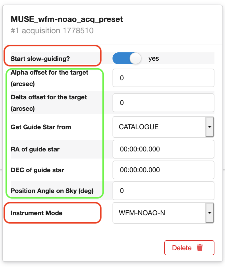
Screenshot of the selected acquisition template.
Parameters highlighted with the red boxes must be defined manually in the acquisition template, whereas those enclosed by the green box can be specified by using ObsPrep.
3. ObsPrep: the Acquisition template
Assuming that you have already partially filled in the Target section with at least the target coordinates RA and DEC, by clicking on the ObsPrep tab, the p2 main GUI appears as follows (note that the screenshots refer to the ObsPrep version in P105; additional functionalities were added later):
ObsPrep Pointing
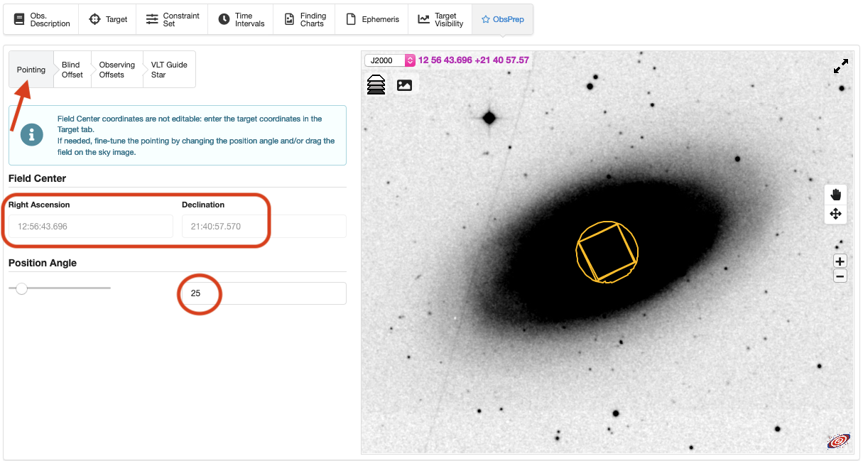
Screenshot of the ObsPrep-Pointing GUI showing the position of the MUSE FoV as defined in the Target section. Note that the coordinates Alpha and Delta (highlighted with the red box), previously defined in the Target section, are automatically propagated to the ObsPrep-Pointing tab (see red arrow), and a DSS image around the pointing is shown in the right GUI. The MUSE WFM FoV and SGS footprint is marked in yellow. You can zoom in/out by using the +/- buttons on the right-hand side of the GUI, or even change the background displayed image by clicking on the picture icon (second icon on the upper left-hand side of the GUI). Should you need to fine-tune the exact target centering (e.g., to make sure that at least one star falls within the SGS area) you can do that directly on the GUI by dragging the yellow footprint on the desiered position (i.e., see the instructions outlined in the blue box), and the tool will update the Alpha and Delta coordinates accordingly in all corresponding fields (i.e., not only in ObsPrep-Pointing tab, but also more importantly in the Target section). Finally, in this tutorial we decide to align the FoV along the galaxy major axis therefore we have set the field orientation to 25 degree by using the Position-Angle (see red circle).
As mentioned above, we are assuming that our science goal is to sample a 3'x1' area on the galaxy's central region, with no particular constraint on the target centring. Therefore, we will not use a reference star for blind offset. Should you need to use the blind offset strategy, here you can find other tutorials explaining how to do it. On the other hand, we want to select a VLT-GS to ensure its compability with the large offsets performed by the OB to monitor the sky background off-target.
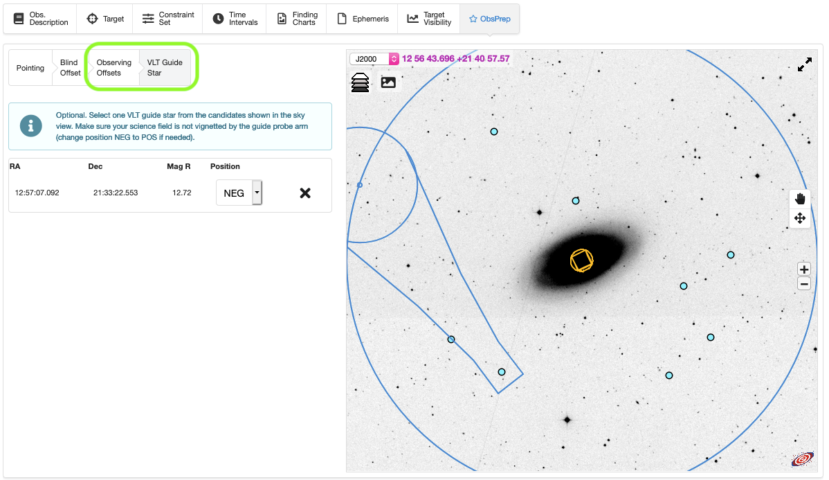
ObsPrep VLT Guide Star
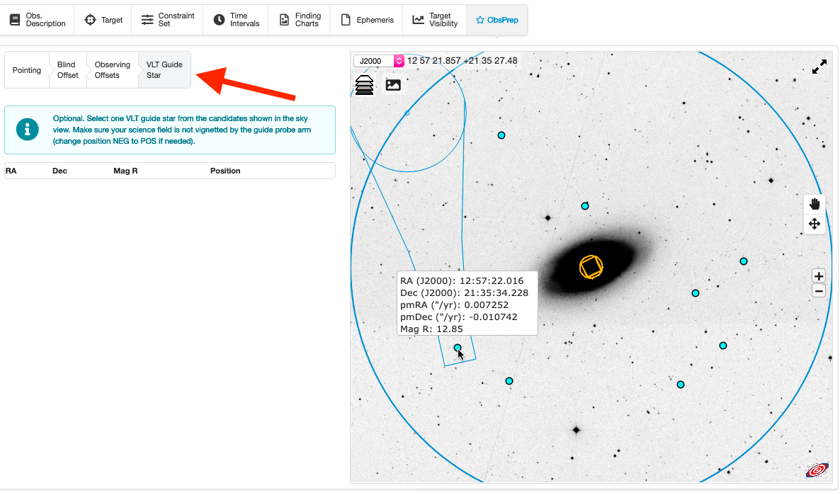
Screenshot of the ObsPrep-VLT Guide Star GUI showing the position of suitable VLT-GSs (cyan big dots, and taken from the Gaia-DR2 catalog) and the telescope patrol field (blue big circle) with respect to the defined target and reference star position. Moving the mouse over any of the marked stars you have access to its position, proper motions and magnitude. In addition, the footprint of the telescope guider arm is also shown in blue.
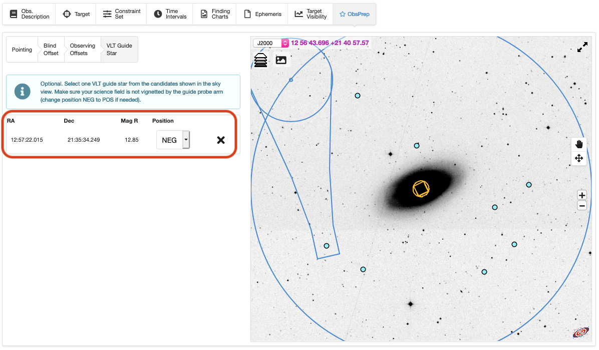
Screenshot of the ObsPrep-VLT Guide Star GUI after having selected a VLT-GS directly on the image. In doing so the tool populates the relevant fields accordingly (i.e., see fields on the left-hand side of the GUI highlighted with the red box). Note: the VLT-GS selection constrains the allowed offsets during the science observations, therefore when the observing strategy requires performing large offsets, it is highly recommended to select the VLT-GS only after having defined the offsets in the science template.
Now, if you go back to the acquisition template under the Obs. Description section you will notice that all relevant template parameters have been properly propagated by ObsPrep (see figure below). Specifically, the RA/DEC of the VLT-GS.
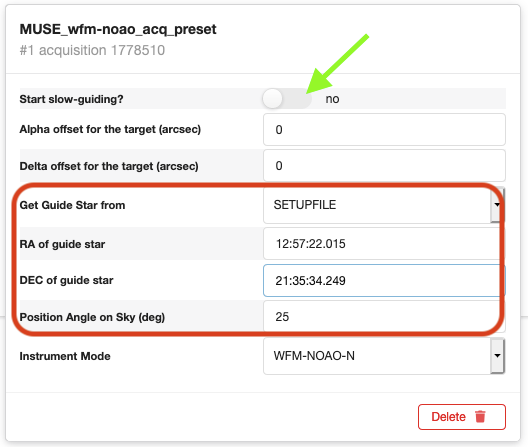
Screenshot of the acquisition template once all relevant information (see red box) has been inserted by using ObsPrep. Note: due to the lack of suitable point-sources in the metrology field, you can disable the Slow Guiding system (see green arrow).
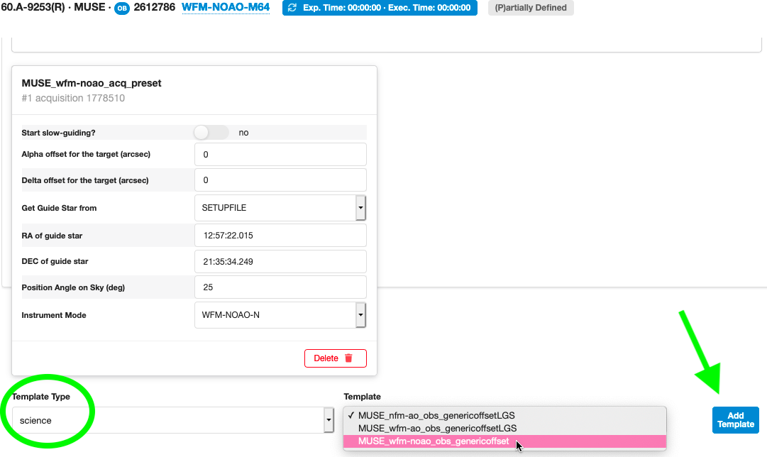
4. Obs. Desciption: the Science template
The only available science template for WFM-NOAO observation is the MUSE_wfm-noao_obs_genericoffset. To load it into the OB, first select the option science in the drop down menu "Template Type", then select the MUSE_wfm-noao_obs_genericoffset from the drop down menu on the right and click on the "Add Template" icon as shown in the figure below.
As for the acquisition case, the set of science parameters appearing on the p2 GUI after loading the MUSE_wfm-noao_obs_genericoffset template can either be defined completely manually or in a more automatic way by using ObsPrep.
In what follows we first provide a short desciption of each parameter, and then we will use ObsPrep to fill in the template.
- Number of offset positions: Number of positions at which you want to take exposures
- Number of exposures per offset position: Number of exposures to be taken at any defined position
- Observation type list, O/S: Each defined exposure must be tagged either as 'O', for on-target observations, or as 'S', for sky monitoring (see sec. 5.4 of User Manual).
- Offset coordinate type selection: The offsets pattern can be defined either in DETECTOR or SKY coordinates system (see sec. 5.4 of User Manual).
- List of relative offsets in position angle (deg): The field orientation at each defined offset position (offsets in position angle are cumulative).
- List of relative offsets in RA or X (arcsec): Offset in RA/X of each defined position (offsets are cumulative).
- List of relative offsets in DEC or Y (arcsec): Offset in DEC/Y of each defined position (offsets are cumulative).
- Return to origin?: This flag is set always to "Yes", meaning that the telescope returns to the original position after the defined offsets pattern is completed. Note that the original position matches the telescope pointing before the science template has started (i.e., after the acquisition). Should you need to set this keyword to "No" you must submit a waiver.
- List of UITs: Integration time (in seconds) of each defined exposure. If all defined exposures must be taken with the same integration time you can just type in a single value.
Note on offsets and field orientation:
To improve the flat-fielding of the slicer and channel patterns during the data reduction we strongly advise the observer to always split the on-target observation in multiple exposures taken at least at two different position angles (separated by 90 degrees) and with a small offsets pattern. The size of each on-object offset should at least be larger than a spaxel (i.e. >0.2" for the WFM).
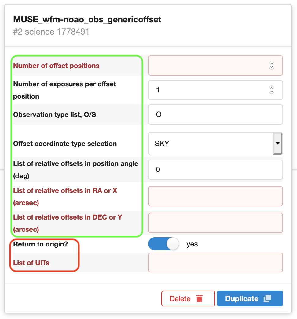
Screenshot of the selected science template.
Parameters highlighted with the red boxes must be defined manually in the science template, whereas those enclosed by the green box can be specified by using ObsPrep.
5. ObsPrep: the Science template
To prepare the science observing sequence we will make use of the ObsPrep. To this end go back to the ObsPrep section and click on the Observing Offsets tab. The main P2 GUI will appear as follows:
ObsPrep Observing Offsets
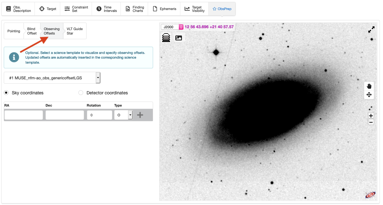
Screenshot of the ObsPrep Observing Offsets showing the target centring. The coordinates reference system for the offsets (i.e., Sky or Detector) can be directly selected in the left-hand side of the GUI, together with the list of offsets in RA, Dec and position angle. The type of exposure (i.e., O or S) can also be defined for each offset.
Because the target is very extended with respect to the instrument FoV to monitor the sky background an off-target exposure is necessary. In addition, to cover an area of about 3'x1' a minimum of 3 adjacent pointings are needed (i.e., a minimum of 3 exposure offset type 'O' separated by ~60"). In addition, to obtain the best results in terms of cosimcs rejection and to improve the flat-fielding of the slicer and channel patterns during the data reduction, we plan to split the total integration time on each of the 3 adjacent pointings into 2 exposures, each one rotated by 90 degrees and taken at slightly different position (e.g., <1"). This strategy leads to a total of 6 exposures on target (i.e., O1 O2 O3 O4 O5 O6) and 1 exposure off-target (i.e., S). Note that the number of exposures and their exposure time should be defined with the help of the ETC to ensure the requested S/N is reached with respect to the total integration time on source.
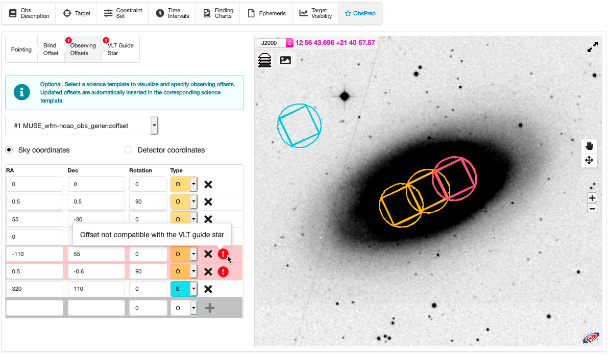
Screenshot of the ObsPrep Observing Offsets GUI showing the position of the MUSE FoV corresponding to the positions defined in the offset list (see left-hand side of the GUI). To define any given offset you must fill in the RA, Dec, Rotation and type fields, and then press the + button next to the offset type field. The instrument FoV footprint corresponding to each exposure is shown on the image. By moving the mouse over any of the defined objects in the left-hand side GUI the corresponding location on the image is highlighted in pink. The red circle symbol appearing next to the 5th and 6th offset highlight a problem with the selected VLT-GS. Therefore, as already anticipated (see above), we must change the VLT-GS.
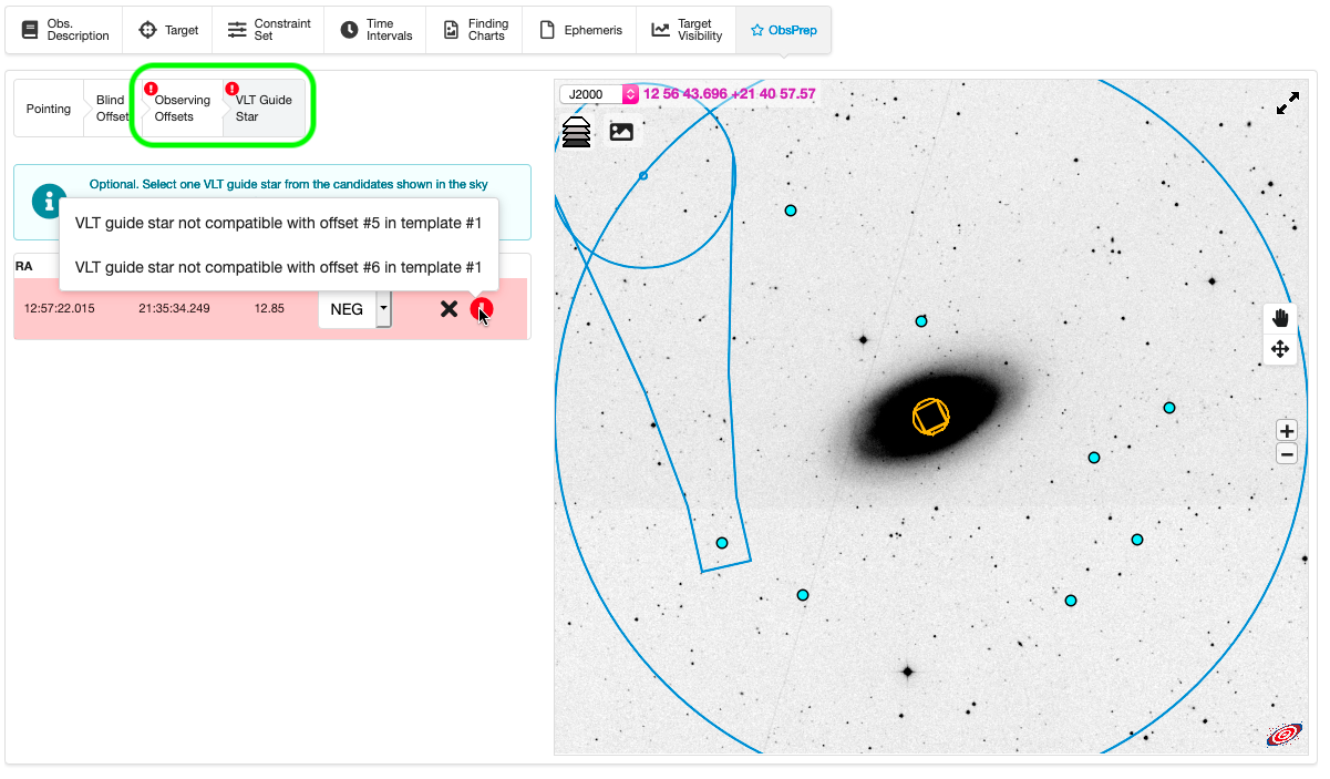
Screenshot of the ObsPrep VLT Guide Star GUI after having selected the observing offsets, which turn out to be not compatible with the previously selected VLT-GS. By moving the mouse over the red big circle you have access to a mini-help window that tells you which of the defined offsets is not compatible with the selected VLT-GS. To change the VLT-GS click on the X button (trash bin in the latest ObsPrep version) and then select another star as done previously.
By selecting a new VLT-GS, all the warnings (i.e., red ! circles) next to the Observing Offsets and VLT Guide Star tabs disappeared (i.e., compare the region highlighted by the green box in this figure and in the previous one).
Now, if you go back to the science template (i.e., in the Obs. Description section) you will notice that most of the parameters have been properly propagated by ObsPrep (see figure below). Specifically, all but the list of UITs that you must fill in manually.
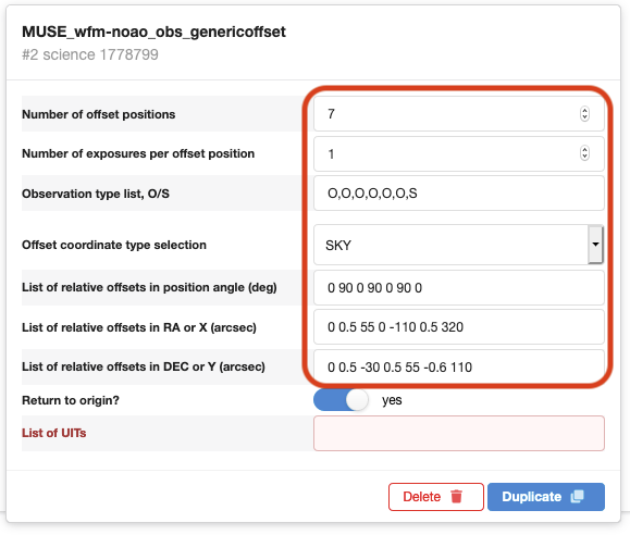
Screenshot of the science template once most of the relevant information (see red box) has been propagated by using the Observing Offsets feature within ObsPrep. Note that the list of exposure times must be inserted manually. In this example, we plan to use the same integration time for all 6 exposures (e.g., 200 sec), and 100sec on sky. Therefore, in the List of UITs field, we must type the following: 200 200 200 200 200 200 100
Finding charts
At this point you must create finding charts compliant with ESO general and MUSE specific requirements. The easiest and quickest way to do that is by using the finding charts generator embedded in the p2 environment. Once the OB templates content has been fully provided, click on the "Generate Finding Chart" button you find under the Finding Charts section. In doing that 2 finding charts will be created and automatically attached to the OBs. Specifically, the tool produces a finding chart showing the position of the selected VLT-GS with respect to the telescope pointing (i.e., large field of view chart showing the telescope patrol field), and a second one showing the MUSE FoV footprint centred on the first object position.

Screenshot of the finding charts created by the Finding Charts Generator. The left image is zoomed onto the target field and it shows the position of the FoV during the acquisition (i.e., red footprint centred on the first pbject position) and during the defined science offsets pattern (i.e., blue footprints shadowed in yellow). The right-hand image shows a zoomed out version of the first finding chart, in which the selected VLT-GS as well as the positions of the telescope patrol field (i.e., big circles) are marked with respect to all defined offsets.
Alternatively, you can provide your own-made finding charts (please consult this page to check all the requirements), which you must manually attach to the OB (i.e., click on the "Upload Finding Chart" button you find in the Finding Charts section).
Access to the final OB
The ascii version of the OB just created, together with the corresponding finding charts can be downloaded here.
Alternatively, by logging into p2 demo, under the programme ID 60.A-9253(R) you can access to the USD-Tutorials folder where this OB have been created and stored. In the same folder you can also find a sample of OBs designed for different modes and observing strategies. The example OBs are not editable but can be exported if needed. Please refrain from creating new OBs in the USD-Tutorials folder.
Instrument selector
MUSE p2 tutorial
- Goal of the run
- Getting started
- OB general sections
- OB instrument specific sections
- Finding charts
- Access to final OB
- Back to MUSE p2 tutorial main page
P2 documentation
Useful links