
ESPRESSO p2 Tutorial
IMPORTANT: ESO is now offering use of the web application p2 for Phase 2 preparation for all Paranal observing runs from Period 102 onward. The web application p2 fully replaces the use of P2PP for the preparation of the Phase 2 observing material for all telescopes/instruments for both Service and Visitor Mode runs on Paranal. Please check our help section about p2 for instructions on how to notify ESO when your material is ready.
This tutorial provides a step-by-step example of the preparation of a set of OBs with ESPRESSO at the ESO-VLT. The specifics of this tutorial pertain to the preparation of OBs for Period 102 onward.
Please note that all the figures shown below can be clicked on to get higher resolution versions.
To follow this tutorial you should have familiarity with p2 : the web-based tool for the preparation of Phase 2 materials. Please refer to the main p2 webpage (and the items in the menu bar on the left of that page) for a general overview of p2 and generic instructions on the preparation of Observing Blocks (OB). Screenshots for this tutorial were made using the demo mode of p2, but should not differ in any way from one's experience in preparing your own OBs under your run.
The example OBs that we will create in this tutorial are available on the p2 demo version, run 60.A-9253(W) - ESPRESSO, in the folder ESPRESSO Tutorial.
0: Goal of the Run
One of the typical science cases of ESPRESSO is the monitoring of the radial velocity of relatively bright stars.
In this tutorial we will prepare a set of OBs that perform the acquisition of a science target and its observation in high spectral resolution with the 1UT mode (singleHR mode) in a time link. This mode provides the highest radial velocity precision down to 10 cm/s.
The example consists of observing the M giant gam Sge (Simbad coordinates RA (2000) = 19:58:45.4282, Dec (2000) = +19:29:31.7273, proper motions RA 65.11 mas/year, Dec 22.73 mas/year), V mag 3.47.
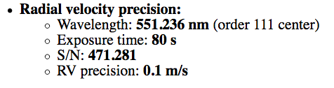
Using this magnitude and relaxed conditions (no moon constraints, airmass 2, seeing 1.2 arcsec), the ESPRESSO ETC tells us that we can expect a radial velocity precision of 0.1 m/s and a S/N of 470 at 550 nm with an exposure time of 80 s:
The monitoring of the radial velocity requires a time link of OBs. For the sake of this tutorial, we will create a time link of 5 OBs to be executed at least 10 days and no more than 20 days one from another.
These sample OBs in a time link will illustrate the use of a variety of features of p2 and the kind of decisions to be taken at the time of preparing in advance an observing run, as well as some aspects that are specific to the preparation of OBs for ESPRESSO.
1: Getting Started
The Phase 2 process begins when you receive a communication of the ESO Observing Programmes Office (OPO) announcing that the allocation of time for the coming period has been finalized and that you can view the results by logging into the UserPortal and clicking on "Check the webletters."
Let's assume you were granted observing time with ESPRESSO in service mode. To start preparing your Phase 2 material including observation blocks, instructions, and finding charts with the web application p2, we recommend you collect all the necessary documentation first:
- The ESPRESSO User Manual
- The ESPRESSO Template Manual
- The VLT Service Mode instructions
- The documentation to the help section about p2 referred to above.
2: Making OBs
2.0: p2
For the sake of this tutorial, we will use the p2 demo facility: https://www.eso.org/p2demo
This is a special facility that ESO has set up so that users who do not have their own p2 login data can still use p2 and prepare example OBs (for example, while writing a proposal to get the overheads right). You cannot use it to prepare actual OBs intended to be executed. When you prepare such OBs you should use your ESO User Portal credentials for p2 (with http://www.eso.org/p2).
After directing your browser to the p2 demo facility the main p2 GUI will appear as follows:
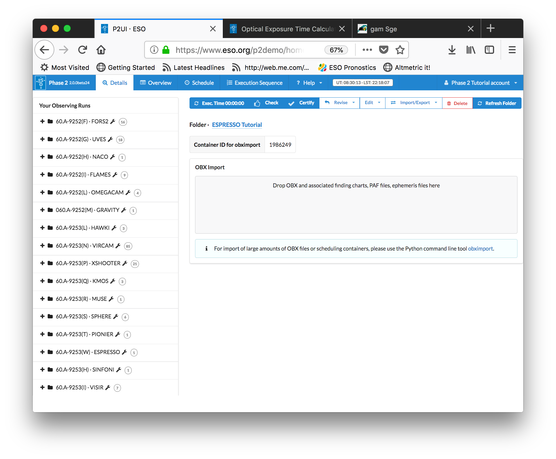
Runs for a number of instruments appear in the left-hand column, since the p2 demo facility is used for all of them. Similarly, if you log into p2 (instead of p2demo) with your own ESO User Portal credentials, you will get the list of all the runs for which you are PI, or for which you have been declared as a Phase 2 delegate by one of your colleagues.
Select the folder corresponding to the ESPRESSO tutorial run, 60.A-9253(W) by clicking on the + icon next to it. In this tutorial we assume that time was allocated in Service Mode. This is indicated by the small wrench icon that appears next to the RunID. "Inside the run" you will see (at least) one folder, called "ESPRESSO Tutorial". That folder contains the final product of the tutorial you are now reading. You can refer to the contents of that folder at any time, perhaps to compare against your own work.
In the p2 demo you must first start by creating a folder, within which you will put your own content.You can create a folder by clicking on the icon New Folder. Please notice that a folder named by default New Folder will appear at the bottom of the list of items in the run. Because the p2 demo is on-line and accessible to anyone you may see folders belonging to other people here, though after-the-fact clean-up is encouraged and possible.
Your screen should look like this after you pressed the "New Folder icon:

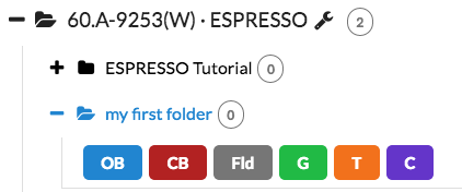
You can give the folder a new name by clicking on the blue New folder text on the top, in this tutorial the name will be "my first folder", but you can set the name of your folder to be (almost) anything you like. Select and open your new folder by clicking on the + icon next to it.
2.1: Creating Containers
Although creating containers is optional in general, ESPRESSO runs to monitor the radial velocity of a source typically make use of a Time Link container, which is a type of container in which OBs are executed with defined time intervals from one to the next. We thus start our tutorial by creating a Time Link container. If you wish to create a standalone OB, please skip this section.
We create Time Link container by clicking on the icon for this type of container, labeled "T" in orange in the icon bar below your new folder:
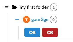
This creates an empty container of type time link in your folder. Again, as for the folders, type a name for your time link container, such as "gma Sge". Your window should then look like this:
2.2: Creating OBs
You can now create your first OB within the time link container "gam Sge": First select your time link 'gam Sge' in the left menu by clicking on the '+' next to it, then press the blue 'OB'-icon below your (highlighted) time link container:
You will now be able to edit the contents of the OB on the right hand side of the GUI. Enter a name just like you did for the name of the folder or the time link.
We start with creating the first OB for gam Sge within the time link and call it gamSge-1. Your screen should then look like this:

In the next steps, we have to edit the OB information. The relevant fields to be edited are organized within the different tabs below the OB name, called "Obs. Description", "Target", "Constraint Set", "Time Intervals", "Finding Charts" , and "Ephemeris" (relevant for moving targets only). A check of the "Target Visibility" on a certain day is also possible.
2.2.1: Defining the Obs. Description
We start with editing the Obs. Description. This tab is already highlighted in blue in the figure above.
2.2.1.1 Filling in the basic information in the Obs. Description
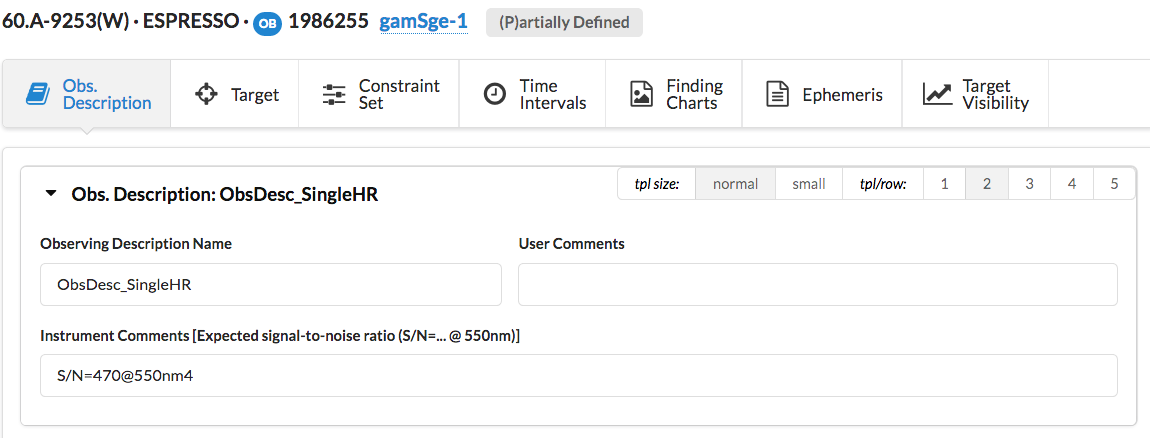
It may be useful in many cases to have an easy way of identifying an observation description, like when having observations of a number of targets performed with identical instrument configuration and exposure times. The Observing Description Name field allows you to fill in an appropriate description. Our example OB is for the singleHR mode. We choose "ObsDesc_SingleHR".
Next, the User Comments field can be used for any information you wish, e.g. to keep further track of the characteristics of the OB, or to alert the staff on Paranal to special requirements. We do not have any special information for our example OB, so that we leave this field empty.
The Instrument Comments field should include the expected S/N. Based on the information from the ETC, we type: S/N=470@550nm
The top of your OB field should then look like this:
2.2.1.2: Defining the acquisition template
The first template that must be part of any OB is the acquisition template, so let us define it next. In the Template Type list, make sure that the acquisition entry is selected. The Template list on the right contains four acquisition templates available for ESPRESSO: those for the HR and UHR modes, and each of these as _obj and _sky. You read in the template manual that the _obj acquisition templates are the only ones offered for service mode, and are for acquisition of objects on sky. We wish to make an acquisition for the singleHR mode, and thus select the template ESPRESSO_singleHR_obj in the Template list, and press the blue Add Template button next to it:
 You need to decide now on the acquisition parameters, which are described in the ESPRESSO template manual.
The first two entries, RA blind offset and DEC blind offset, refer to a blind acquisition from a reference star, which we do not need for our bright target gam Sge. We thus leave these values at 0.
The next three entries, Telescope guide star selection, RA of telescope guide star, and DEC of telescope guide star, refer to the choice of the telescope guide star. We do not have any certain requirements for the guide star, and leave the values at their defaults, which means that the guide star will be selected at the telescope from a standard catalogue.
We then enter the properties of our source gam Sge:
- Object color index B-V: 1.57
- Object V mag (this is a mandatory input): 3.47
- Guess Radial Velocity (km/sec): -34
- Object spectral type: M0
- Object redshift: 0
The acquisition template should then look like this:

2.2.1.3: Defining the science exposure template
In the TemplateType list, select "science", We select the "ESPRESSO_singleHR_obs" template and click Add Template. After editing the values the window should now look like this:

,The best options for our case are:
Binning/Readout mode: 1x1_FAST
Source on fiber B: FPCS
Calib. associated fiber A: ThAr (note that the LFC is currently not operational, see the instrument news),
and we also enter our exposure time from the ETC calculation:
Exposure time: 80.
This completes the filling of the Obs. Description.
2.2.2: Setting the target information
Click on the Target tab at the top of the OB view window in order to insert your target name, coordinates, and proper motions. The fields Differential RA and Differential Declination are used for differential tracking (solar system objects, for instance), and in our case we leave them with the default values of 0. The acquisition template including the target information is now complete, and the Target view should look like this:

2.2.3: Defining the Constraint Set
As stated in Section 1, we assume for the purposes of this tutorial that the program has been allocated time in Service Mode. You thus need to specify a set of constraints which indicate under which conditions your OB can be executed.You can do this by clicking on the Constraint Set tab on the top of the OB window.
Constraints Name:
First, give a descriptive name to the constraint set about to be defined. Since you have decided that this constraint set will be applied to all the observations using the singleHR mode, you type for example "Constr_SingleHR" in the Constraints Name field.
Note that in your Phase 1 proposal you already specified some of these constraints (sky transparency and seeing) according to the requirements of the ESPRESSO instrument webpage. You must make sure that none of the constraints specified in Phase 2 is more stringent than the corresponding ones specified at Phase 1.
Airmass:
We used an airmass of 2.0 for our ETC calculation. We thus enter 2.0.
Sky transparency:
Since our target is bright, observations can be done with THIN conditions, and enter "Variable, thin cirrus".
Lunar Illumination and Moon angular distance:
We did not use moon constraints for our ETC calculation, as our target is bright. We enter 1 and 30 deg, respectively, corresponding to no moon constraints.
Image quality:
The ETC tells is that our Phase 1 seeing constraint of 1.2 arcsec corresponds to an image quality of 1.5 arcsec, so that we enter 1.5.
Twilight:
This parameter defines whether or not the observation can be extended into twilight. We decide to leave the default value of 0 min.
PWV:
We read in the user manual that this parameter shall only be used for special requirements in the red part of the spectrum. We leave the default parameter of 30 mm.
Your Constraint Set tab should now look like this:

2.2.4: Defining Time Intervals
Click on the Time Intervals tab at the top of the OB window. Here you can add both Absolute Time Constraints (left tab) and Sidereal Time Constraints (right tab):

Both kinds of time intervals are optional. Absolute Time Constraints can be used to allow execution of this OB only within the windows specified, for example if the observations have to be coordinated with another facility, or if it shall happen during an eclipse. Sideral Time Constraints constrain the local sidereal time at which the observations shall be executed within any given night.
To help with the definition of absolute time intervals, there is a chart available that shows times that are blocked for other purposes than service mode. Note that your run is pre-scheduled on a certain UT, and that the chart shown corresponds to that UT. However, any of your observations may be re-scheduled during the period to another UT. As a result, please make sure that your observations are feasible with the schedule of your pre-assigned telescope, but at the same time as broadly defined as scientifically possible to allow a flexible scheduling withint he period.
We do not have any such requirements for our observations, and thus do not add any constraints.
Note that the relative time intervals between our OBs within the time link container are not set here, but in the Schedule view at the very top of the window. We will come back to this later after we have finished the OB.
2.2.5: Attaching Finding Charts
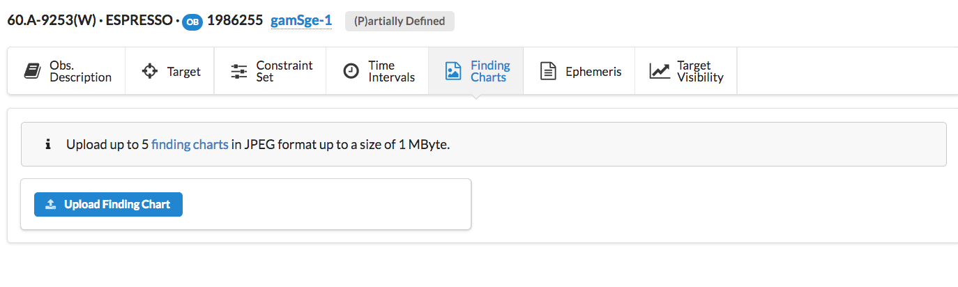
The final step of preparing the OB is to attach a Finding Chart. The Finding Charts must be prepared as jpeg-files and must fulfill all general and ESPRESSO specific requirements for finding charts. You can use any tool of your choice to create the Finding Charts in jpeg-format.
Let's assume you have prepared a jpeg-Finding Chart for this tutorial run [remember: run ID 060.A-9253(W)], which you called 060.A-9253W.gamSge01.jpg, and which is saved in a sub-directory of your home directory.
In the Finding Chart tab, click the blue box Upload Finding Chart, and select the Finding Chart on your disk:
This completes the creation of our example OB for gam Sge.
2.3: Completing the concatenation and verification
Now, with the first OB of our time link container completed, we need to add the remaining OBs. Since all of the observations are identical, we can simply select our OB gamSge-1 in the left menu and use the option Edit -> Duplicate OB to create the other four identical OBs:

We name the five OBs gamSge-1, gamSge-2, gamSge-3, gamSge-4, gamSge-5, all under our time link container gam Sge:

We now click on the Schedule button in the very top horizontal bar of the p2 window, and enter for each OB after the first:
Earliest after previous: 10d
Latest after pervious: 20d
The Schedule view should then look like this:
 Before submitting the time link container to the ESO data base, please check it by first selecting the time link container gam Sge in the menu on the left, back in the Details view, and then clicking the Check button (the one with the thumb-up icon). To certify the concatenation and the OBs, press the Certify button. This will indicate to ESO that the concatenation is ready, and you will not be able to modify it anymore. After you have finished the complete material under your own run ID, including the ReadMe and the Checklist, the last step would be to go back to the top-level run in the left menu, and to press the Notify ESO button at the top.