Common DFOS tools:
Documentation

make printable | back to: phoenix description · process instances

Find here a detailed overview of the characteristics of the MUSE_DEEP PHOENIX process. The focus is on specific properties for this instance. The standard PHOENIX process is covered here. Find the phoenix tool documentation here.

Phases of the DEEP phoenix process:

• preparation
• processing (phoenix -P)
• certification (phoenix -M)
• post-processing

Aim of MUSE_DEEP

Many MUSE runs aim at going deep. This is evident from the abstracts, and from the observing patterns. A run that has a 1-hour OB on a target and another couple of identical OBs for the same target is quite typical. Each OB might accumulate 2-4 individual exposures, which are combined by the normal MUSE PHOENIX process into one combined datacube. However, each visit (OB) of the same target produces another such datacube, while the real goal of the data reduction would be to combine all input frames in one single combined datacube. The purpose of the MUSE_DEEP project is to combine all such multiple target visits in one deep datacube per target.

Number of OBs and exposures	1 OB, N=1 exposure	1 OB, N=4 exposures	>=2 OBs
product: single datacube			...	single datacubes are always available, indirectly offered as S. files
combined datacube			...	one datacube per OB: available as combined MUSE datacube
deep datacube				one datacube per target: MUSE_DEEP datacube
process	MUSE_R		MUSE_DEEP

Red background: final datacube, offered as MUSE phase3 product
Blue background: final datacube, offered as MUSE_DEEP phase3 product
Open symbols: available as S. files only; filled symbols: available as IDP

If a target has been observed in only one exposure, then the single datacube is the final product; if only one OB exists (but more than one exposure), then the combined datacube is the final product. If there is more than one OB per target, the deep datacube is the final product (but the combined datacubes continue to exist from the MUSE project, they are not hidden or overwritten).

The main motivation for going deep is based on these two arguments:

• the scientific usefulness of a deep datacube is much higher than for the N combined datacubes individually, because the limiting magnitude is better for the deep datacube;
• for the archive user, it is quite demanding to process the deep datacube because of memory requirements (see below).

The MUSE_DEEP processing is executing on muc11 (as muse_ph3) because this is the most powerful machine available (56 cores, 2 TB memory). The preparation is executing on muc10 (as muse_ph2) because this is the MASTER of the MUSE_R process, collecting all information.

Preparation (as muse_ph2@muc10): phoenix_getInfoTarget; phoenix_getInfoRun and phoenix_createDeep

phoenix_getInfoTarget

The tool $DFO_BIN_DIR/phoenix_getInfoTarget is used only exceptionally, in complex situations: several different runs observe an overlapping set of targets. The overlap in general is only partial. This situation is quite common among GTO runs. Then, the list of PI/CoIs often (but not always) is identical, as is the proposal title. The tool, if called for one runID, then finds the overlapping targets, and from there the ovelapping runIDs. The tool is iterative, and can thereby also analyse complex situations. The output is a text file with the full list of targets, indicating in which runs they have produced observations and datacubes. This output list is very useful for several situations: decide which run should become the MASTER and which remain SLAVEs; define partial releases; double-check whether a target has been observed in other runs or not.

Be aware of the fact that the tool uses the target name as given by the PI. In case of existing datacubes, this target name may have been modified, then the QC1 database name is used.

Always double-check the output list (target - runIDs) for completeness and correctness.

The tool is called like

phoenix_getInfoTarget -r "run_ID" (on the command-line, for a given run_ID; brackets included!)

The output list is displayed on the terminal.

phoenix_getInfoRun

This is the main tool to create the overview of periods, runs and targets. It is running automatically, once per day as a cronjob on muc10. It takes as input the complete history of the MUSE_R processing. The information relevant to the MUSE_DEEP project is collected under the path ~/monitor/FINISHED/RUN.

The tool is called like

phoenix_getInfoRun -r "run_ID" (on the command-line, for a given run_ID; brackets included!)

or

phoenix_getInfoRun -A (for all runs, as cronjob).

The tool information sources are the QC1 database entries in muse_sci_combined. Every final datacube created by MUSE_R is registered there.

The tool creates the main overview page, with one line per run, which has all information relevant for the decision if a run is eligable for the MUSE_DEEP combination. It is linked to the dfoMonitor on muc10, under 'RUN_IDs (local)', pointing to

~/monitor/FINISHED/RUN/overview.html.

For each period, there is a summary table with run overview information.

For each run, there is a detailed table with all processed datacubes.

The tool is exporting the file RUN_TYPE.txt (see below) to the DEEP processing site muse_ph3@muc11 where it is read by the phoenixMonitor. The opposite is true for the file DEEP_MODE.txt that is filled by phoenixMonitor and is scp'ed from muc11 to muc10. (While phoenix_getInfoRun is a helper tool specific for a particular project, the tool phoenixMonitor is a general phoenix tool. This setup is probably not stable and might evolve in the future.)

Period overview tables

There is one period overview page per period. These are the columns of the period overview tables:

Status tables

Under the same path there are three status tables which build the "memory" of the run review process.

• RUN_DATA.txt: this table is entirely managed by phoenix_getInfoRun. The tool discovers new runs by scanning the QC1 table muse_sci_combined and adds them to the RUN_DATA.txt table. It checks and updates the status information. In particular it evaluates the processing completeness. This table is updated every day through the cronjob. There is no need for the user to interact with this table.
• RUN_TYPE.txt: this table is entirely maintained by the user. If a new run is entered, the user decides about the type (C: crowded,M: mapping, D: deep, S: dynamic sequence, O: other), whether to combine as DEEP (YES/NO), and can enter comments. The type value is for information only. C might remind the user to mark this run as CROWDED in the latter stage of the process (see under phoenix_createDeep). M, O and S would not qualify for DEEP combination.
• RUN_MULTIPLE.txt: this table is used to mark runs which logically belong together (partially overlapping set of targets). Very often (but not necessarily!) they share the same PI, the same programme title and the same abstract. All such runs together form a coupled set of targets, called "multiple runs". For the DEEP combination, it is important to collect all files common to a target in the same pool. Formally, such coupled runs seem to be against ESO policy but this is the observed behaviour for many GTO runs.

The status tables play an important role for the creation of the DEEP runs.

Run overview tables

For each run_ID found in RUN_DATA.txt, all entries in muse_sci_combined are collected and transformed into an HTML table, which has the following columns:

The table comes as enhanced table, it can be sorted and filtered, in order to offer a comfortable way for target selection. If a run has OBJECT and SKY observations, these are color-coded, then there is also a separate HTML page with the objects only. The FOV previews are extremely useful for the target selection. If you filter by a target name you see immediately whether or not the FOV is the same. Usually one can expect that the same target name implies the same FOV and then constitutes a case for DEEP combination, but there are also cases when a target name has not been chosen "good enough" and there are different pointings with the same target name.

On top of the run overview table, find additional information and links to:

• abstract and run information,
• pointings (QC1 plotter link with all RA and DEC as found in muse_sci_combined for that run),
• ABMAGlim plots to single, combined and deep results (deep makes sense only if the DEEP processing has been done already),
• SKY_RES plots for single and combined results,
• if the run has been marked as DEEP run (see below), there is also a link 'targets' for the final target selection,
• 'all_runs' links back to the period overview page.

On top of that, there is an overview of the other linked runs if this run is multiple, and a link called 'target search'. That link goes to the output page of a 'createReport -Q' run which however is not automatically created but needs to be called by you on a command line, case by case. It might be very useful if you want to explore the data reports for a given target name, or run_ID, or in general any pattern. The output page is then easily found behind that link.

Creating a new DEEP run

On the period overview table, you find candidates for a new DEEP run as follows:

• normally you proceed period by period;
• naturally you should not create a DEEP run before it is USD-completed, and before its processing is completed;
• there is no exact rule when to do it but a common-sense rule is that runs from the current period cannot yet qualify for such a review;
• many targets have limited visibility over the year so it is generally wise to wait at least about one year before a qualifying run is marked as DEEP;
• for runs with files older than a year, the abstract becomes visible which is a valuable source of information;
• initially a new period has no identified DEEP runs;
• you look for candidate runs that are COMPLETE in terms of processing, and have a USD run_status COMPLETE, TERMINATED or CARRY-OVER. VM runs unfortunately have no such flag but are safely finished if the observing dates are 'old enough'. This might not be true for GTO runs which might have several periods of observing nights.

For a candidate run,

• go to the run overview page,
• check the abstract (for key words 'deep', 'multiple' etc.),
• use the 'target' column for sorting and filtering and check the FOV images,
• double-check at the bottom that there are no entries 'Yet to come'.

If there are multiple lines with the same FOV, they usually qualify for DEEP combination (unless they represent a dynamic sequence).

If you decide to mark a run as DEEP,

• enter a new line in RUN_TYPE.txt with the run_ID, VM or SM (just copy), mark the type as appropriate (likely is D or O), 'YES' to combine (important!), and a comment as appropriate;
• call 'phoenix_getInfoRun -r "run_ID"' again.

If you decide that this run should definitly not be combined, enter a line with a 'NO' in column #4, and call the tool again.

If you want to enter a comment but not decide yet, enter a line with 'TBD' in column #4, and call the tool again (or wait for the cronjob to do this for you eventually).

Target selection page

If you have entered 'YES', you should visit the run overview page again after refreshing the tool. You will now notice a new link 'target' on the top navigation. Click this link and find the target selection page.

On that page, all targets of the run that have at least two entries (corresponding to two datacubes to combine) are displayed, separated by a line for better grouping. Single datacubes are shaded slightly different than combined datacubes. The columns are the same as on the run_ID overview page, but the table is now sorted by target name. Click the link 'sortable' to go back to the run_ID overview, and click 'txt' for the target overview text file. This file is important since it controls the final target selection. Line by line, it has the same columns as the html page, but is has more lines, some of them are commented out. These are the lines with a single OB.

The text file is created in a completely automatic way, and it is created only once, upon the first execution of the tool after marking a new run with COMBINE=YES. Afterwards, the text file serves as reference for the target selection, and for the datacube selection. If the automatic datacube selection needs to be refined, you can comment or un-comment lines. The new selection will be taken into account upon the next execution of the tool. Hidden or unhidden entries will be considered in the html overview page. Critera for the selection or deselection could be the OB grades, seeing values, OB comments or other circumstances.

Likewise, you can fine-tune the target combinations. Column #4 in the text file has the target name. By editing it (e.g. from NGC300 to NGC300_P1 for one subset, and to NGC_P2 for another subset if you need to collect two different pointings), you can fine-tune the target combinations. The new combinations will be taken into account after the next execution. Note that in principle you are free to choose whatever TARGET name you want, it is not checked against the header keys.

Target selection for multiple runs

If you have marked runs to belong together, their overview text pages will be combined. This brings together all input for a given target, no matter if it comes from run #1 or from run #2. It is strongly recommended to check the combined text file for cases where in the individual text files a target would have only one entry line and get commented out, but in the combined file would have more than one entry. You would then need to unhide both lines in order to make the target active.

If a MASTER run is still collecting, set the COMBINE flag in RUN_TYPE.txt to TBD. If a .txt file already exists (e.g. because you initially did not know that this would become a complex MASTER/SLAVE combination), delete it. If you finally decide to release, set COMBINE to YES, and you will find all candidates for OB combination from all MASTER and SLAVE runs in the MASTER .txt file.

Preparing the ABs: phoenix_createDeep (as muse_ph2@muc10)

If you have done the target selection for a new run, start the collection and creation of the ABs, using the tool

phoenix_createDeep -r "<run_ID>".

This is an interactive tool that is only executed on the command line.

It works with the target overview text file. For each of the targets selected there, it

• scans the QC1 comments (in order to discover previous issues with the data which might have led to rejection),
• finds all single OBJECT datacube entries and downloads their corresponding ABs (sci_basic ABs and sci_post ABs, extension pst),
• adds all SKY ABs if existing,
• creates an exp_combine AB with all pst products.

No shallow datacubes are created.

All downloaded information is collected in $DFO_AB_DIR/TMP2. The downloaded ABs come from the MUSE_R branch on qcweb which is the final storage for the products of the MUSE IDP processing. The exp_combine AB is formally identical to a tpl AB, but in order to avoid confusion with the existing OB-based tpl ABs, it gets the extension 'dpc' (deep combine).

You will be asked if the data are in CROWDED field mode. Contrary to the MUSE_R project, the crowded field nature of the target is now known in advance from the QC reports, so that the processing parameters can be optimized for that case. If an exposure is taken of a crowded field (globular cluster), without dedicated sky observations, then the default sky determination strategy of the MUSE_R IDPs is the determination of the sky from the data, which, because of the nature of the fields, may lead to an overestimate and an oversubtraction of the SKY. This can be avoided here by answering Y. (If dedicated SKY observations exist, then answer 'N' since the subtraction of an external SKY is always ok.) For Y, a field will be added in the ABs (PROC_MODE=CROWDED) which will later be interpreted by phoenix.

Also, the TARGET name will be added to the dpc AB, and in case of multiple runs, the formal RUN_ID of the master will be added to the dpc AB.

After all this editing, you can inspect the collected, edited and created ABs before they get uploaded to qcweb, this time to the new branch MUSE_deep. This will be the AB source for the MUSE_DEEP processing. Note the difference between MUSE_deep (input for DEEP processing) and MUSE_DEEP (output of MUSE_DEEP logging).

This is the last step for the preparation of a run_ID for MUSE_DEEP processing with phoenix.

Selection strategies

If a PI designed 10 OBs of 4 exposures each, which all where executed in Service Mode under 0.5 arcsec seeing while the constraint was 0.7 arcsec, and all OBs were graded A, the strategy for combination is obvious: combine them all in a N=40 dpc AB. This is what the target selection overview file will indicate, and what will be reflected in the FOV previews.

A number of situations is not so clear. In VM, in particular for GTO runs, many OBs are executed partially, to adapt to the prevailing conditions. To get them automatically selected by the selection tool is rather reliable but needs a consistency check nevertheless. Then there are rare cases when an exposure was aborted (after say 120 sec while the regular ones took 300 sec). This exposure will add more relative noise than the others, hence it is a candidate for rejection.

OBs graded C might be candidates for rejection as well but not necessarily. In particular, there are a few cases when an OB has been graded 'C' once, and a second time 'A'. The A datacube might likely be better than the C datacube. But since both exist already as MUSE IDPs, adding a third one, deeper than either of them, is a good idea, since then archive users can make their own decision which one to choose for their science. An example is the DEEP datacube for 095.B-0934A.

Generally it seems worth to de-select only extreme cases of bad seeing (or other constraints). Moderate deviations from the constraints are acceptable, as can be seen in some cases from published results where PIs combined all input data accepting even OBs graded C.

Photometric instabilities can be ignored except for extreme cases when an exposure was aborted.

Rather often, when the natural size of a target does not match the 1'x1' FOV of MUSE, targets are observed e.g. in a 2x2 pattern, with overlaps of say 20% only. It is then a matter of taste whether one wants to combine all input exposures in one deep datacube, with the overlapping regions benefitting from a factor sqrt(2) (and even a factor 2 in the central part) enhancement of the SNR, or in 4 separate deep datacubes. This choice can be controlled by setting the target name in the overview text correspondingly. There is also the memory limit on the number of input exposures (about 120).

Carryover: if a SM run is granted carry-over status by USD (meaning it has been closed initially and then is opened for more OBs to be executed in the next period again), the automatic collection of the new datacubes by phoenix_getInfoRun works fine. Just make sure to release the run not too early. Usually the carry-over decision is made before the end of a period.

Large Programmes: those SM runs that extend across several periods collect fine and complete with phoenix_getInfoRun. Just make sure to wait with the call of phoenix_createDeep until the end of the last period.

"Multiple" runs (GTO): enter all runIDs in RUN_MULTI.txt, and all observations of the "SLAVE" runs will be collected in the "MASTER" run by phoenix_getInfoRun.

Other little tools for the AB preparation

Processing: phoenix (everything from here on as muse_ph3@muc11)

When working with phoenix for MUSE_DEEP, you always work on a run_ID, or on a selected AB of a given run_ID:

Like for MUSE IDPs, it is not possible to call the phoenix tool for MUSE_DEEP IDPs without option, because the certification review is mandatory.

The tool downloads all ABs that have been put by phoenix_createDeep onto qcweb (MUSE_deep), including all dpc ABs, or the specified dpc AB only.

pgi_phoenix_MUSE_AB_deep

The phoenix tool works with standard dfos components plus with instrument-specific PGIs. For MUSE_DEEP the first PGI is

The MUSE_DEEP science cascade is a bit simpler than for MUSE. In particular we need:

• the single OBJECT ABs (extension .ab, recipe muse_scibasic) and the muse_scipost AB (extension _pst.ab);
• if any: the single SKY ABs (extension .ab, recipe muse_scibasic) and the muse_create_sky AB (extension _sky.ab);
• the dpc ABs (only OBJECT) are duplicated into a muse_exp_align AB (extension _dal.ab) and the muse_exp_combine AB (extension _dpc.ab).

The different types of ABs can be recognized by their extension. Note that the dpc ABs are formally the same as the tpl ABs (same recipe, same processing parameters) but have the extension dpc (deep combine) for safe distinction against the tpl ABs. The dal ABs (dal stands for deep alignment) are formally identical to the tal ABs. They are created by the PGI from the dpc ABs.

There are two different cases for the processing scheme, either without SKY or with SKY observations:

a) N OBJECT frames, no SKY:
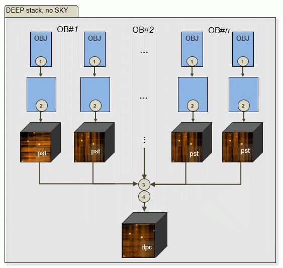	Output of PGI: per target N scibasic ABs, N scipost ABs, one exp_align AB, one exp_combine AB. N is only limited by memory, currently to about 120. The number of OBs doesn't matter.
b) N OBJECT frames and some (M) SKY frames:
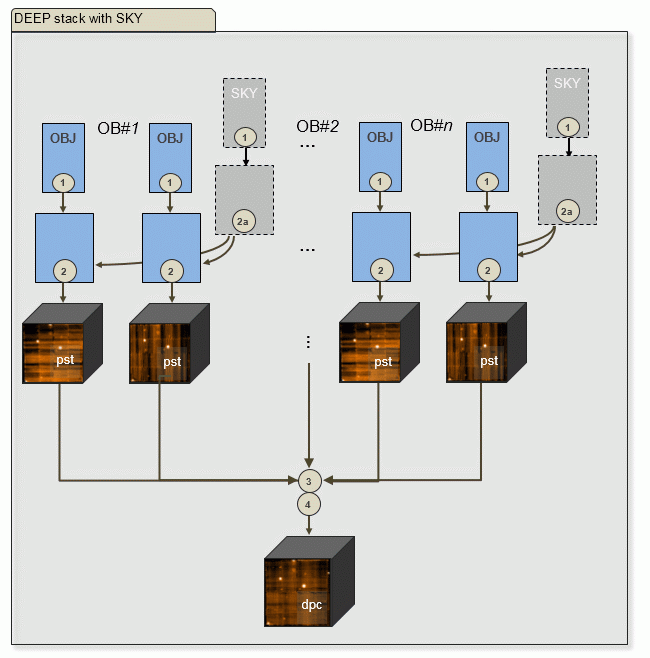	Output of PGI: per target M scibasic ABs for SKY, M create_sky ABs, N scibasic ABs, N scipost ABs, one exp_align AB, one exp_combine AB. M is usually smaller than N. The number of OBs doesn't matter.

There is no combination of SKY ABs into shallow datacubes.

Based on the information entered by the user during phoenix_createDeep, the tool knows about PROC_MODE=CROWDED. It applies two different sets of processing parameters, for the cases CROWDED or 'not crowded':

All master calibration associations come by AB/OB and are not modified. No new associations are created. All processing of scibasic, create_sky and scipost ABs has been done already in MUSE_R but it is repeated here, because no PIXEL_TABLE products have been stored in the first pass. Neither are they stored here, because

• they are big and would not fit onto the 10 TB hard disk;
• storing them in NGAS would blow up the archive significantly;
• creating them from scratch is possible with a moderate investment of compute time: with 3-stream processing on muc11, one such pixeltable takes about 3-10 min.

After execution, all ABs are in the standard $DFO_AB_DIR, ready for execution.

Processing: pgi_phoenix_MUSE_stream

The JOB_ PGI is the same as for MUSE_R, pgi_phoenix_MUSE_stream. On muc11, 3 streams are enabled. This is the execution scenario:

If there are no SKY ABs, we start with the OBJECT ABs (#3).

Compute performance

The required processing time on muc11 is dominated by the dpc AB which, very roughly, takes about the same time as all other ABs together. Its processing time roughly scales with the number of input pixel_tables to be combined. An N=100 dpc AB (which is among the biggest and rarest ones) takes about 20-24 hours and about 1.6 TB of memory.

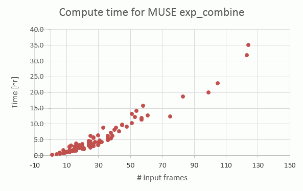	Empirical relation between number of input pixel_tables (frames) and processing time for the exp_align recipe, on muc11
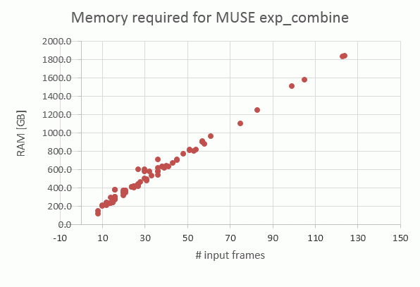	Same, for the memory. On muc11, with the 2 TB of memory available, we can combine up to about 125 input files.

What if:

-- the dal (exp_align) AB fails, causing the dpc (exp_combine) AB to fail:

• check out the formal reason for failure; if it was 'input file not found', this likely means that a previous pst AB failed (this rarely happens because of unknown memory issues); if true, re-execute the scibasic and the scipost AB, then try the dal AB again;
  • before you then try the dpc AB again, inspect it: very likely the OFFSET_LIST file is now commented out, this needs to be undone before executing the dpc AB again (otherwise it would execute without the alignment);
• if the dal AB still fails, or if it failed for a different reason (presumably on working on a particular pixel_table):
  • modify the parameters (make the threshold smaller) until it succeeds
  • then check the dpc AB as described above before executing.
• if nothing helps: the input dataset might contain a wrong input file, with a pointing not overlapping with the others;
  • then check again the target overview pages for that target: if you can identify an outlier, just comment it out and proceed as above
  • you can also run processQC on all pst ABs and inspect the QC reports, in order to find some anomaly.

- the dal AB executes fine but the alignment correction is bad (as visible in the QC plot):

• is this a crowded field, and you have forgotten/decided against PROC_MODE=CROWDED: try running the dal AB again, with modified parameters as recommended for CROWDED mode
  ( --iterations=20000. --threshold=100. --srcmax=200 --srcmin=2 --step=5.)
• inspect/visualize the alignment table:
  • cp <dal.fits> ~/midwork/
  • inmidas-->indisk/fits; cre/grap; set/grap xaxis=-0.001,0.001 yaxis=-0.001,0.001; plot/tab <dal.tbl> :RA_OFFSET :DEC_OFFSET; [copy/grap postscript; $lp -d pacolm10 postscript.ps]
  • if there is an outlier: eliminate (in dal and dpc AB!) and process again
  • if not, modify parameters to better cluster
• useful for verification: with the modified dal.fits, call the dpc AB with --lambdamin=5100 --lambdamax=5600 or similar, executes within 15 min for N=48, check the result with rtd. Don't forget to disable these parameters before final execution.

- the QC report of the dpc AB shows some input files with very different flux:

• likely better to drop it from the list (in dal and dpc AB) and reprocess it (because the scaling approach of the pipeline makes sense only if the scale differences are not too big).

- the dpc AB runs out of memory: this seems to be an issue with the alignment recipe for certain input coordinates (for muse/2.2):

• this might occasionally happen because the dal AB claims a bogus high correction value (like 1e8 degrees instead of the usual 1e-5 or so), and the dpc recipe interprets this to reserve the corresponding huge grid;
• the issue then is with the dal recipe and its product; inspect the dal result table (inmidas -P; read/tab ...): is there a coordinate outlier? It might be due to a numerical instability in the recipe, which you can explore by playing with the processing parameter 'threshold': make it smaller, execute, check the result table: if now all exposures give reasonable results, execute the dpc AB again with this stable alignment table, it should work now;
• if this is not possible: remove the offending pixel_table in the dal AB, try again;
• if this doesn't work: disable the dal product, try again the dpc AB;
• if this doesn't work: no more options.

Note:

• The processQC calls create a new QC report and a new score for the pst ABs, overvwriting the existing one from the MUSE_R processing. This is done for simplicity and also in order to have the flexibility, to optimize or modify the processing parameters (and thereby the QC1 parameters). This has been used so far only for the CROWDED field mode.

Certification: phoenixCertify_MUSE

After finishing the 'phoenix -P' call, the products are (as usual) in $DFS_PRODUCT, waiting for certification.

The certification tool phoenixCertify_MUSE is configured as CERTIF_PGI. It is the same as used for MUSE IDPs. It can be called stand-alone on the command line, but normally it is called by the third step of phoenix, after processing:

For MUSE_DEEP, only the dpc ABs are reviewed. For a quick check of the pst ABs, click the coversheet report and see them all. The coversheet also contains the MUSE_R tpl ABs for comparison (these are the historical ones). There is the usual comment mechanism. The PATTERN is alsways DEEP, followed by the number of combined frames.

The standard ERRORs and WARNINGs are the same as for MUSE_R. There is one additional WARNING, the one for abnormally high background. This occasionally occurs for CROWDED field processing. There is no standard way of handling this.

If you want to enter a comment about a specific pst AB, use the 'pgi_phoenix_GEN_getStat' button on top of the AB monitor.

In the CROWDED processing mode (sky subtraction turned off), the rare cases of OBs executed too close to the dawn exhibit an excessively high background. In the normal processing mode this gets subtracted and corrected (though the result might be negative fluxes). In the CROWDED mode no correction is applied, and the overly high background might corrupt the deep datacube. This becomes visible only through the QC system, which discovers cases with very high background and flags them with a comment "High_background". Best strategy is to identify all exposures of that OB (or the ones affected), remove them from the dal and the dpc ABs, and execute the combination again.

Certification: the QC system

The MUSE_DEEP QC system has the following components:

• QC procedures;
• QC parameters, QC databases;
• Scoring system;
• QC plots.

All follow the standard DFOS scheme.

QC procedures. There are two QC procedures (both under $DFO_PROC_DIR):

• qcpar_PIXTABLE_OBJECT_DEEP.sh (for products of pst ABs),
• qcpar_PIXTABLE_REDUCED_DEEP.sh (for products of dpc ABs)

(note: the names are historical, they have no particular meaning). Both are derived from their MUSE_R counterparts. They are largely similar but differ when dealing with the additional properties for the combined datacubes (products of dpc ABs). They feed the QC parameters into the QC1 databases, derive the score bit, and call the python procedure for the QC plots. The qc1Ingest calls for the QC1 parameters are stored locally, under $DFO_PROC_DIR, as qc1_PIXTABLE_OBJECT.dat and qc1_MUSE_DEEP.dat.

QC parameters, QC databases. The QC parameters are generally speaking all kinds of parameters that might be useful, not only for QC, but also for process monitoring (e.g. PATTERN, score_bit), research on science cases (PROG_ID, abstract links) etc. They are fed into three QC1 databases:

• muse_sci_single
• muse_sci_deep
• muse_sci_sources.

The first two are rather similar in structure and collect data for the single and deep-combined datacubes. (The existing entries for the single datacubes are overwritten.) The third one collects parameters for every pipeline-identified source and could be used to monitor alignment quality etc.

Scoring system. There are two aspects of the scoring system:

• the scores as known in the DFOS system
• the score_bit string as written into the product headers and available to the users.

There are 7 scores for single datacubes (pst ABs), they are the same as for MUSE_R.

There are 3 scores for the deep-combined datacubes (dpc ABs):

• offset: indicates if no offset correction was applied at all, or if the correction was larger than normal;
• number_src: to indicate anomalies like 'no sources found' or 'too many sources found'; this score has no practical meaning;
• time_range: the time range in days spanned by the first and the last OB in the datacube; this score has no practical meaning.

Since the MUSE pipeline is very "tolerant" with failures at intermediate steps (where other pipelines would just fail), it seems useful to monitor e.g. the size of the output datacube, or check for complete processing.

While the output of the scoring system is used for certification, and is stored locally but not exported to the user, the score_bit is used to give the user some indication about the data quality. It consists of 10 binary values (0 or 1) coding product properties in a very concise way. They are documented here and in the release description. They are automatically derived by the QC system and written into the product headers as key QCFLAG. The scores are identical to the ones for combined datacubes, except for #11 (MODIFIED) which has no meaning for deep datacubes.

QC plots. Each product datacube gets its QC plot which is ingested into the phase3 system and gets delivered to the user. They are created by the python routine muse_science.py under $HOME/python.

Post-processing: pgi_phoenix_MUSE_moveP

After certification, the standard phoenix workflow takes place (calling moveProducts). There is a pgi within moveProducts, pgi_phoenix_MUSE_moveP, the same as for MUSE_R, but its actions are much simpler and more standard. All deep datacubes and their FOV images are collected under $DFO_SCI_DIR/<pseudo-date>.

After phoenix: conversion tool idpConvert_mu_deep and ingestProducts

After phoenix has finished, all science products are in $DFO_SCI_DIR, all logs in $DFO_LOG_DIR, and all graphics in $DFO_PLT_DIR. This is the standard architecture also known from DFOS.

The final call is 'ingestProducts -d <pseudo-date>' which for MUSE_DEEP has two parts:

• conversion of IDP headers with idpConvert_mu_deep,
• phase3 ingestion of IDPs and ancillary files with IngestionTool@call_IT.

In order to prepare for IDP ingestion, the IDP headers need a few modifications. This is the task of idpConvert_mu_deep. (Every IDP process has such an instrument specific tool, with the instrument coded in its name).

The ingestion log is in the usual place known from dfos: $DFO_LST_DIR/list_ingest_SCIENCE_<date>.txt.

The conversion tool adds ASSOC, ASSON and ASSOM keys to define the IDP dataset, consisting of the IDP (deep datacube, named MU_SCBD), its ancillary fits file (IMAGE_FOV), ancillary text file (pipeline log), and ancillary graphics (QC reports). See more in the release description.

Note: the pst.png files are included in the IDP datasets for completeness, but they exist already under the same name as ancillary files for the combined datacubes. This would not be accepted by the ingestionTool. Therefore their names are converted into 'pst1.png'. In rare cases it might happen that a given 'pst1.png' file has already been ingested for an earlier deep datacube but needs to be associated to a second deep datacube. This cannot be discovered by the conversion tool. It raises an error for the ingestionTool. In those cases, call idpConvert_mu_deep again (by hand), with the parameters '-d <pseudo-date> -p pst2'. The graphical files will now get their names ending with pst2.png. The ingestion should then follow by 'call_IT' (or as 'ingestProducts' with the conversion tool temporarily disabled in the config file).

After finishing, the tool has

• created $DFO_SCI_DIR/<date>/conv,
• moved all IDP fits files and ancillary files (IMAGE_FOV) there,
• filled a text file CONVERTED which is used by ingestProducts to recognize the data as converted.

The products are then ready to be phase3-ingested with ingestProducts.

The call of ingestProducts and, afterwards, cleanupProducts is usually done in the same way as known from DFOS_OPS:

• there is the job file JOBS_INGEST (linked to the dfoMonitor) that is filled by phoenix with all new ingestion jobs; just call it;
• after successful ingestion, there is a new entry in the cleanup job file which you then also call, upon your convenience.

The successful ingestion is displayed on the phoenixMonitor, in the 'DEEP' part, sorted by periods and run_IDs.

Note that for MUSE there is the CLEANUP_PLUGIN needed (pgi_phoenix_MUSE_cleanup) that manages the proper replacement of all ingested fits files (IDPs, ancillary) by their headers.

Other little tools

There is a number of little tools for all kinds of special tasks. If possible they were configured with standard mechanisms in the standard DFOS tools or in phoenix. Their naming scheme follows a standard when they are specific for phoenix: they start with pgi_phoenix, then follows either MUSE or GEN. Unless otherwise noted, they are stored in $DFO_BIN_DIR.

Scheduling. A MUSE_DEEP phoenix job is always launched manually. It always requires the preparation of the ABs with phoenix_createDeep on muc10.

Note that the MUSE-DEEP tasks (AB processing) check for "foreign" autoDaily tasks (currently of espresso) and wait for them to be finished (see above).

Other links

History: http://qcweb/MUSE_DEEP/monitor/FINISHED/histoMonitor.html

Release description: under http://www.eso.org/sci/observing/phase3/data_streams.html.

Monitoring of quality: On the WISQ monitor, there is a monitoring of ABMAGlim vs. exposure time for MUSE and for MUSE-DEEP. There is also QC-reports and scores on individual products. -reports and scores

Terms and keywords: