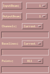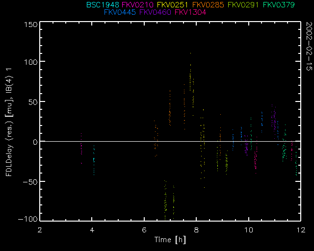

Therefore, we begin hierarchical editing bad data first by looking at the delays (relative to the reference station) of delay lines/stations one through six. The plot widgets as shown below are created using Reduce|PointData|Astrometry|PLOT. The one on the left is the general plot selection widget. The one on the right, the (data) index selection widget, is created when additional input is required as to the indices of the selected data. Create it by selecting "FDLDelay (res.)" for the Y-axis variable. Note that this image is clickable; use it to learn the function of some of the buttons!.
Now, set all the fields just like in the widgets shown below. Remember to terminate your entry in a text field with <return>!

We can see immediately what looks like to be three scans on BSC1788 and BSC1931 without tracking. Use Util|Edit (located in plot selection widget) to place three rectangular boxes around the bad data points and flag them. Then use Pl/E|Auto to automatically flag outliers in this plot of delay versus time for station E02. Then plot these data again. They should look like this.

Do this for all other stations too by selecting the appropriate InputBeam (IB) number. Note that, in contrast to station E02 (IB 1), the delay data for BSC1931 with station AC0 (IB 2) is good! Also note that with station W01 (IB 5), there is some bad data on FKV0460 around 11 UT which is a bit easy to miss. Remember that InputBeam 4 is AW0, the reference station, for which the delay is identical zero by definition.

Use Pl/E|Auto to flag outliers for all baseline of output beam 1 and 2. This step further eliminates bad tracking data. Spectrometer 1 should then look like this:

After removal of bad data caused by bad fringe tracking, we now turn to removal of data due to bad NAT (i.e. narrow angle) tracking and detector problems. We have to skip the former step though since the NATCounts data is not available for this night. (In the context of hierarchical editing, NATCounts have the same effect as FDLDelay.)
Instead, we continue with plotting the PhotonRate, which is the total number of photons recorded on average per 2 ms instrumental coherent integration time. Select OutputBeam 1 and channels 1-4 (make sure you terminate your channel selection with a "return" and that the channels directive is set to "Selected"). This plot should be created.

We notice right away that there is something wrong with the data from FKV0291, which is Procyon (Alpha CMi). Checking the observer log (click on Utilities|List|ObsLog beginning with the main OYSTER widget) indicates problems with clouds and temporarily knocked-out APDs due to the large brightness of this star. Even though we do not plan on reducing the data for this star, you could exercise your editing skills by removing these data. Just select "Time" for the Y-axis, and plot only data for FKV0291 (star directive set to "Sel" and this star highlighted in the star list). Then plot and use Util|Edit to manually place a single large box around the data points plotted, and flag the data. When you return to the PhotonRate plot (remember to set the star directive back to "All"), the bad PhotonRate data of Procyon should have disappeared. You may now run all channels of the two spectrometers through Pl/E|Auto (Note added in proof: skip this and the remainder of the editing steps as too much data would be removed making the imaging exercise too difficult!).
Finally, we want to make sure that no (unexplained) bad squared visibility amplitude data remains, and there we select all stars, channels, baselines, and use Pl/E|Auto. Notice that about 2700 data visibilities are flagged in OutputBeam 1, and 1400 in OutputBeam 2. This is less than two percent of all data, since in this data set there are about 1500 integrations, 16 channels, and 6 baselines per spectrometer.
If, at this point, you are unsure about how your editing was and the state of the data, you may want to use a previously prepared flag table on freshly restored data. For this do the following.
get_points
Allocated arrays for 62 scans in 2 ob's; MB = 6, MC = 16, MP = 1498
Reference station set.
Dispersion corrected delays initialized.
Data loaded.
Reduce|PointData|Flagtable|Load
Reduce|PointData|Flagtable|Apply
The first command reads the PointData (i.e. the 1 s averages) again, the
last two widget buttons restore and overwrite the existing flag table with
one provided on disk (2002-02-15.flg), and then applies the flags to the data.
You are then ready to continue with the bias corrections.
Continue