
OYSTER keeps track of these incoherent scans, and the bias widget procedure described below only processes those scans.
Before averaging the data for the bias computation, we need to set the background counts to zero. Type at the OYSTER prompt:
defaultbg
Default Backgroundtable created.
Default Background data set.
average
Averaging rates and squared visibilities...
% Compiled module: MEAN.
% Compiled module: MOMENT.
Averaging triple products...
Averaging delays...
Finished astrometry computations.
Finished visibility estimation.
Finished averaging.
We now use Calibrate|SYSTEM to bring up a special plot widget for system calibrations. It is shown here. (The Bias button and Points directive are clickable fields for more information.)
In addition, the bias coefficients depend on the number of beams falling on the detector. These different configurations can be selected using the binary fields listed in the Points selection. Fit coefficients are only stored if such a sub-array configuration is selected to make sure they were derived with a well defined setup.
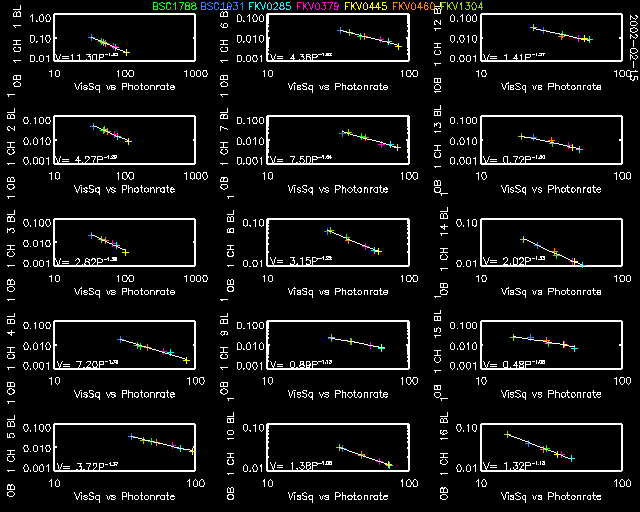
With the data selection as shown above, plot bias fits for all 16 channels of baseline 1 of outputbeam 1, which should look like this:

There is no need for these exercises to plot in such detail all the
other fits, so select all baselines and channels and plot the results
for the two spectrometers and both configurations. Even though the
scale of the plots will prevent you from studying the exact fit results,
only by plotting them will the fits be perfomed and stored in the
appropriate system calibration tables.
After this has been done, reload the background data (remember that we had to set the background rates to zero for the bias computation).
get_bgdata
Backgroundtable created.
Background data loaded.