Modelling Seeing

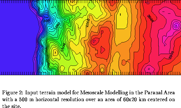
 Following earlier attempts by [Bougeault 95] of a mesoscale model applied on a mountainous continental site, a feasibility study has been started by [Masciadri 97] for the Paranal area using the recently developed meso-nh model including slight modifications appropriate to optical turbulence modeling. The model is non-hydrostatic, and as such allows the vertical development of orographic waves which are believed to be responsible of a large part of the nighttime tropospheric seeing. Such waves indeed create areas with high kinetic energy (and thus well mixed air) at the boarder of which strong vertical gradients of the potential temperature constitute sheets of high optical turbulence.

One of the possible outputs of such a 3-D model, shown on Fig. 6 could obviously be useful during site surveys to exclude areas potentially unfavorable such as the immediate vicinity of the steep coastal chain.
 

 

Tuning a model such as meso-nh is a complicated task because two parameters have to be minimized: the modeling error and the operational cost. Table 5 clearly illustrates the challenge. The cheapest configuration would allow several runs per night to be performed in an operational manner, while the two highest costs would simply forbid any operational use. Initial results of the study by [Masciadri 97] show that a simulated time of 30 minutes is often not sufficient to fully resolve terrain-atmosphere interaction, it is thus reasonable to assume that the cost of a simulation will be of the order of a few hundred DM.

 

Area Vert. Res. Horiz. Res. Simulated Time Time Step CPU Time Price

(km) (m) (m) (sec) (sec) (sec) (DM)

$$60\times 20 500\times 500$$ 300 1800 2.5 4629 1388

$$60\times 20 500\times 500$$ 600 1800 2.5 1945 583

$$60\times 20 1000\times 1000$$ 300 1800 5 719 215

$$60\times 20 1000\times 1000$$ 600 1800 5 296 88

$$60\times 60 500\times 500$$ 300 1800 2.5 13219 3965

$$120\times 120 2000\times 2000$$ 600 1800 10 400 120