v=fringevis(bincounts(1,*,*,*))
v2=fringevissq(bincounts(1,*,*,*))
help,v,v2
V COMPLEX = Array[32, 42300]
V2 DOUBLE = Array[32, 42300]
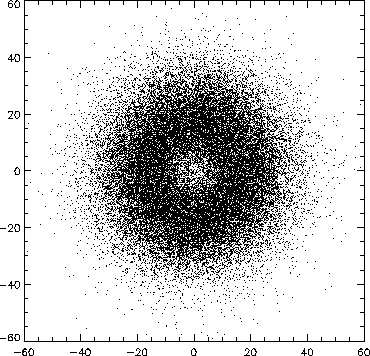
A complex variable has real and imaginary parts, they can be plotted as follows.
window,xsize=400,ysize=400
plot,float(v(0,*)),imaginary(v(0,*)),psym=3,xrange=[-50,50],yrange=[-50,50]

window_slide plot,v2(0,*),psym=3

Using the observer star and obs log sheets to figure out which tracking was selected and which stations were pointed at the star, I check whether I find fringe frequency peaks at positions (i.e. values of k) consistent with that information.
Here is the configuration information from which we can see what baselines correspond to which values of k:
print,genconfig.stationid
	E02 AC0 AE0 AW0 W07 AN0
print,genconfig.fringemod
           7           1           6           5           2           8
           5           3           7           4           1           8
print,genconfig.baselineid
      E02-AE0 AE0-AW0 AN0-AW0 AN0-AE0 E02-AN0 E02-AW0
      E02-AC0 AC0-AW0 W07-AW0 W07-AC0 E02-W07 E02-AW0
The fringemod parameter indicates the values of k, the first line above
corresponding to the first spectrometer. The baselines by spectrometer
are also given above.
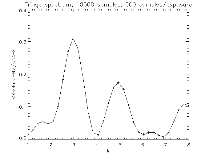
Here is the fringe frequency spectrum for scan 6 on 2001-10-16 while E02, AC0, and AW0
were tracking a star. The spectrum below shows that we indeed see peaks
at k=3 (AC0-AW0), 5 (E02-AC0), and 8 (AW0-E02)

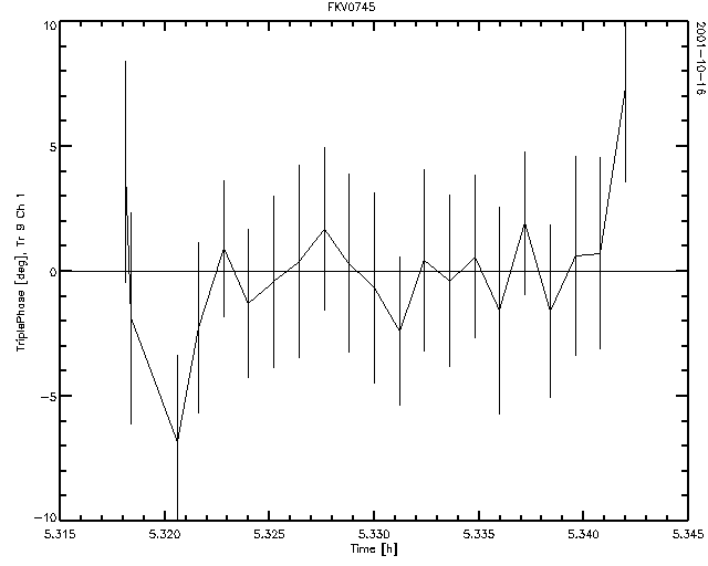
The one-second averaged closure phase derived for the three
baselines in this spectrometer is shown below. It is of good
quality and clearly free of atmospheric phase noise.

The third baseline occurs twice in this configuration, and the same
triple, but in a sense independent from the first one, can be
computed and is shown here.
