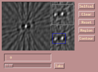
 This is the PEARL widget. It is a clickable map for explanations of the maps
and buttons.
set_complexvis
pearl,'FKV0497'
The first command creates complex visibilities from the observed squared visibility amplitudes and closure phases.
 This is the PEARL widget. It is a clickable map for explanations of the maps
and buttons.
 Before we begin, we have to self-calibrate the data to a point source
(click on "Selfcal").
Also, we define a region
(click on "Region").
as shown with an arbitrary effective temperature (and
log(g)) of 4000K and 4.0. Since we define only one region, the exact numbers
do not matter. Notice that the CLEAN slider is not active.
Note that the region is set to not
include the faint component on the other (right)
side. Since we began self-cal with a point source, this component is an artefact
which will disappear as soon as we pickup flux from both components in the
defined region. Had we placed the window incorrectly over the other pair, the
algorithm would not have converged since the data would have been
inconsistent with the closure phases.
 If we grab the slider, after a
brief delay
it will be movable and we can study the
changing residual and final maps as a function of the number of CLEAN components
subtracted. These components are green colored pixels in the residual map, and
we chose to set the slider to 32 since this was about the highest number of CLEAN
iterations before components would be subtracted at positions other than the two
locations corresponding to the stars in this binary.
 Using the "Take" button,
we add the selected number of CLEAN component to the
current model (which was empty at the start), self-calibrate the phases, subtract
the CLEAN components from the data, and re-display the updated residual and final
maps. The CLEAN slider moves back to zero for a new cycle of hybrid mapping.
 After a few iterations, there is nothing more left to CLEAN aside from side-lobe
structure and noise. Click on "Contour", and a map similar to the following should
be displayed.

 The phase data is now calibrated and tradition has it to throw out the model and
start over with the calibrated data to see if we missed any structure outside
the regions we defined at the start (which is unlikely here since we are looking
at an ordinary double star rather than a radio quasar with a long jet, for example).
Use the CLEAR button to clear the model. Then remove the old region (use "Region",
right-click on final map, the select "Reset". Redefine a region about the size of
the map. The result is shown on the right.
 The final image and map. Notice that you may not get the same result, and that the
quality of the maps varies. PEARL as implemented in OYSTER does not yet take
data weights into account, so there is room for improvement. If you want to see
how the map visibilities fit the observed visibilities, you have to read in the
provided model file using
readmodel,image.model
calcmodel,
which just uses the star_model.mode parameter to tell OYSTER that it is
a map (rather than e.g. a limb darkened disk) to transform.
Next section