Apus: ESO CCD Test Report
EEV 44-82 -1-A57
CCD name : Apus
Serial number :
9252-14-02
Type : Backside, Single layer AR Pixel size 15x15 µm
Number of photosensitive pixels 2048 x 4102 [HxV]
Number of
outputs : 2
Overall rating :
Test date : 02/11/2000
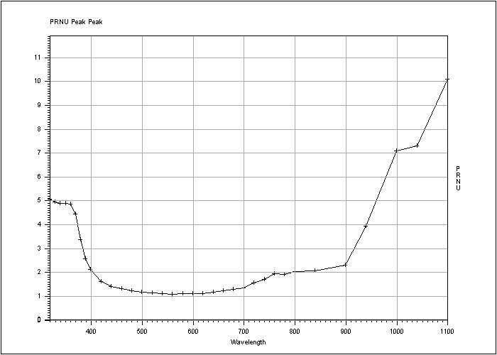
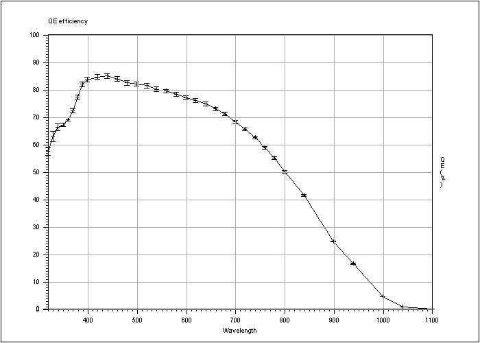
Clock mode: EEV 1p/225k/HG 512
Conversion Factor= 0.53746e-/ADU ±0.001545 for 24744.9ADU
RMS noise = 3.7507e- ±0.1753


CCD temperature : -120.0Cº


Window area is : X1= 64 X2= 2093 Y1= 4 Y2= 507
Bandwidth 5nm

Wav. QE% PRNU rms% Phase=
320        57.5     ±1.6         5.05            7.006147
330        62.9     ±1.8         4.93            6.979452
340        66.2     ±1.3         4.88            6.968215
350        67.1     ±0.66        4.89            6.970295
360        69.1     ±0.68        4.86            6.966696
370        72.3     ±0.71        4.42            6.869861
380        77.2     ±0.76        3.35            6.593095
390        81.9     ±0.84        2.56            6.321791
400        83.6     ±0.85        2.11            6.124742
420        84.6     ±0.85        1.61            5.846838
440        84.9     ±0.85        1.4             5.694374
460        83.8     ±0.84        1.32            5.633757
480        82.4     ±0.83        1.21            5.539744
500        82       ±0.82        1.17            5.509408
520        81.4     ±0.82        1.13            5.483239
540        80.1     ±0.81        1.1             5.458051
560        79.4     ±0.58        1.08            5.44497
580        78.2     ±0.78        1.1             5.462481
600        76.9     ±0.76        1.09            5.463989
620        76       ±0.75        1.11            5.483575
640        74.7     ±0.73        1.15            5.528542
660        72.9     ±0.71        1.22            5.583677
680        71.1     ±0.68        1.29            5.648755
700        68.2     ±0.64        1.35            5.681619
720        65.5     ±0.6         1.54            5.805105
740        62.5     ±0.57        1.7             5.869988
760        58.8     ±0.53        1.92            6.003469
780        54.9     ±0.48        1.91            5.971177
800        50       ±0.43        2.01            6.043367
840        41.4     ±0.35        2.04            6.063942
900        24.6     ±0.2         2.28            6.120477
940        16.5     ±0.13        3.94            6.724411
1000       4.55     ±0.034       7.07            7.286271
1040       0.715    ±0.0053      7.28            7.313993
1100       0.0772   ±0.00057     10.1            7.710604
Table 1: Measurement of the Quantum Efficiency.
Figure 1: Graphic representation of the QE.
Figure 2: Graphic representation of the PRNU.
In this section you can compare the QE we measured with the testbench and
QE Minimum specification
Typical QE
QE from Marconi
Figure 3: Comparison between the QE measured by ESO, the QE measured by Marconi,
ESO specification and minimum specification.
|
Comparison QE ESO / QE Marconi |
||||
|
Wavelength (nm) |
QE ESO (%) |
QE Marconi (%) |
Difference (Eso - Marc. %) |
Relative difference (Marconi as reference %) |
|
350 |
67.1 |
58.3 |
8.8 |
15.1 |
|
400 |
83.6 |
82.1 |
1.5 |
1.8 |
|
500 |
82 |
81.2 |
0.8 |
1 |
|
650 |
73.8 |
73.8 |
0 |
0 |
|
900 |
24.6 |
28.5 |
-3.9 |
-13.7 |
Table 2: Difference and relative difference between ESO measurement and Marconi.
Figure 4: Graphic representation of the difference and the relative difference.
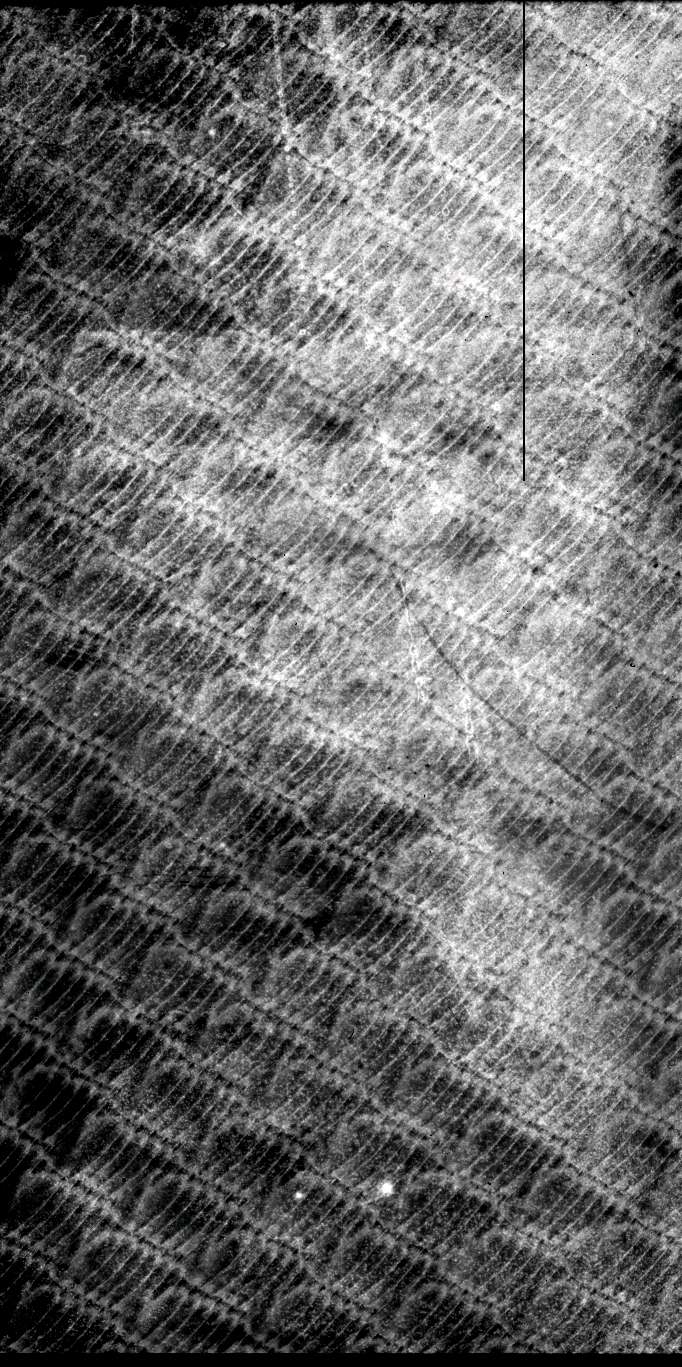
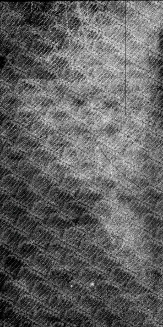
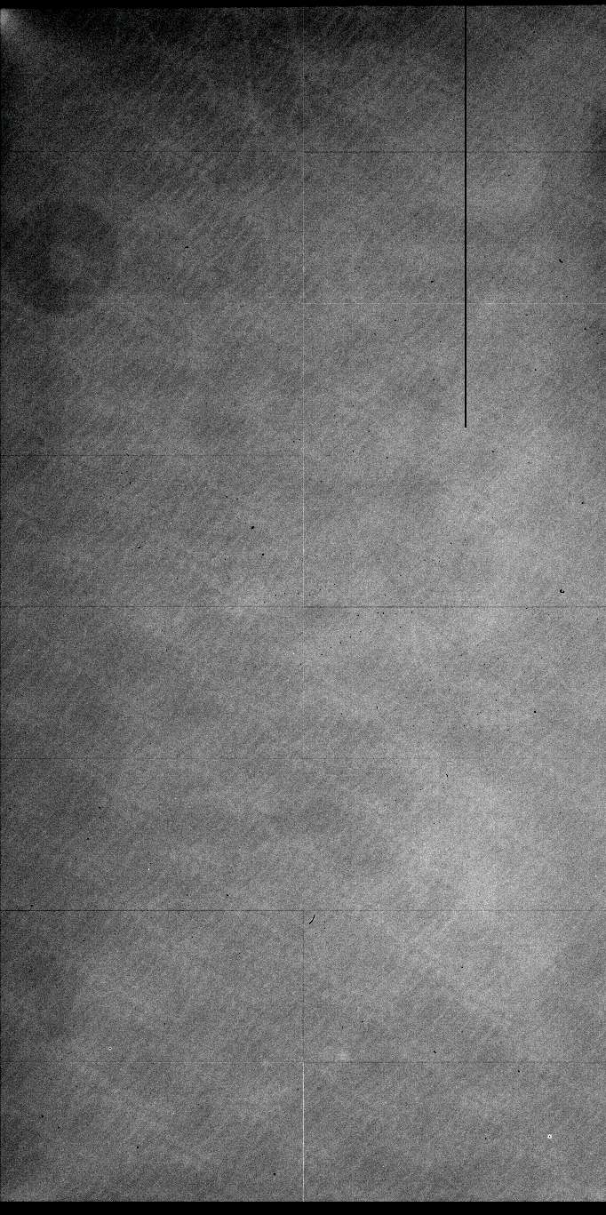
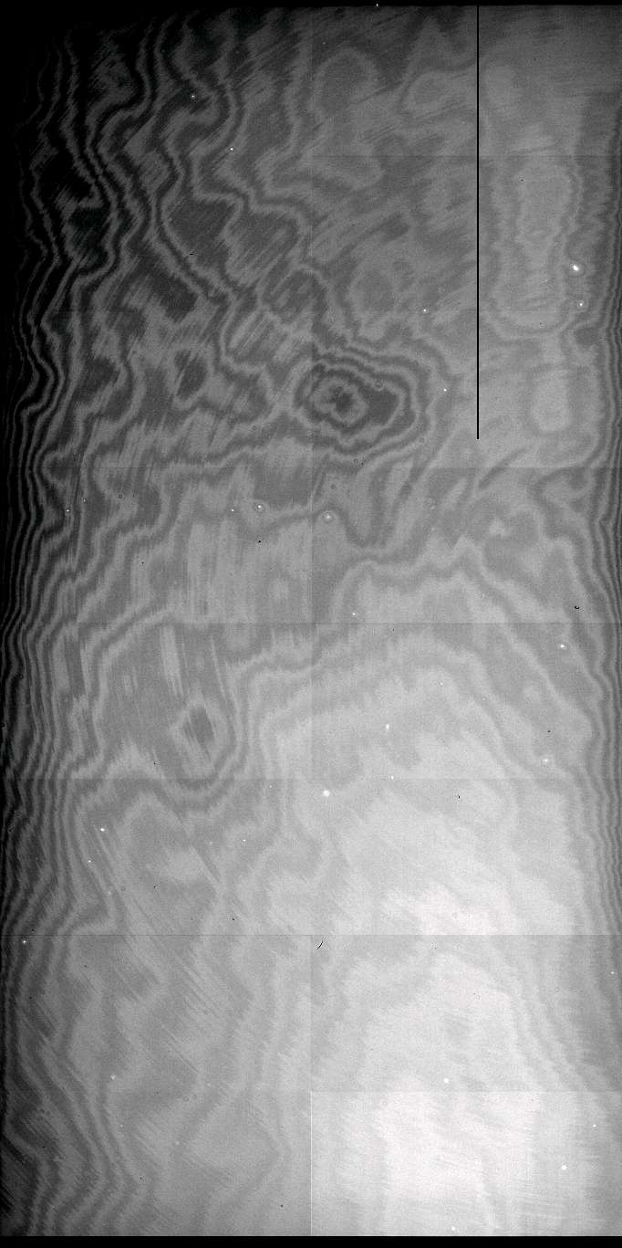
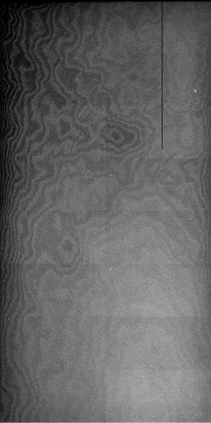
For the flat field we use three wavelengths, 350nm, 600nm and 900nm. For each wavelength we make two images, high level (45000 ADU) and low level (1000 ADU).
350nm (UV), bandwidth 5nm |
600nm, bandwidth 5nm |
900nm, bandwidth 5nm |
|||
|
|
|
|
|
|
|
High level |
Low level |
High level |
Low level |
High level |
Low level |
Table 3: Flat field for three wavelengths.
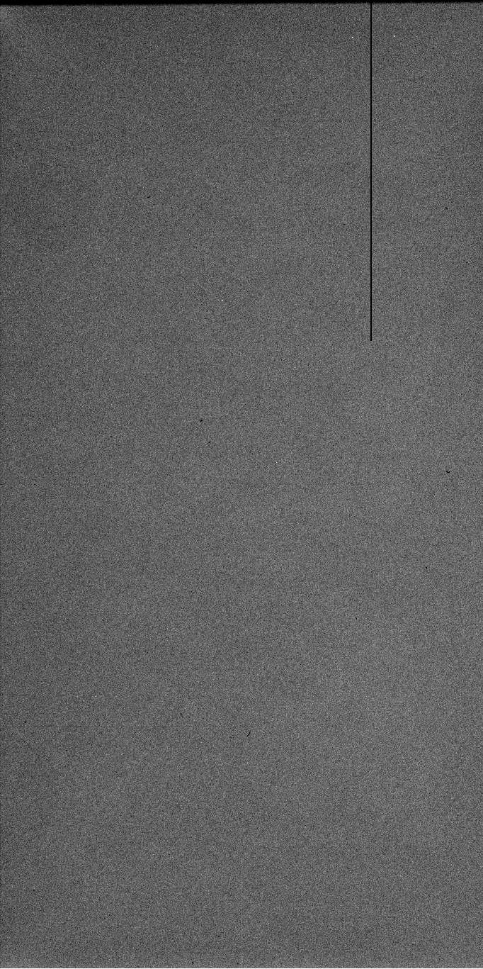
The time exposure, for the long dark exposure, is 3600 seconds.
|
Bias |
Long exposure dark image |
|---|---|
|
|
|
Table 4: Bias and dark.
Readout speed: 50kps
Right readout port
Conversion Factor= 0.432e-/ADU ±0.001 for 27266.4ADU
RMS noise = 2.9e- ±0.2

Left readout port
Readout speed: 50kps
Conversion Factor= 0.556e-/ADU ±0.002 for 26601ADU
RMS noise = 2.5e- ±0.2

Readout speed: 225kps
Right readout port
Conversion Factor= 0.418e-/ADU ±0.002 for 20909.6ADU
RMS noise = 4.0e- ±0.3
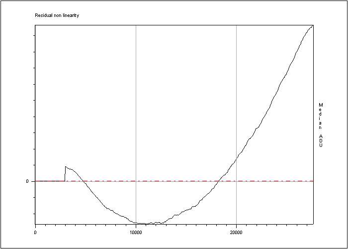
RMS non linearity (%) = 0.201357
Peak to peak non linearity (%)= 0.629146
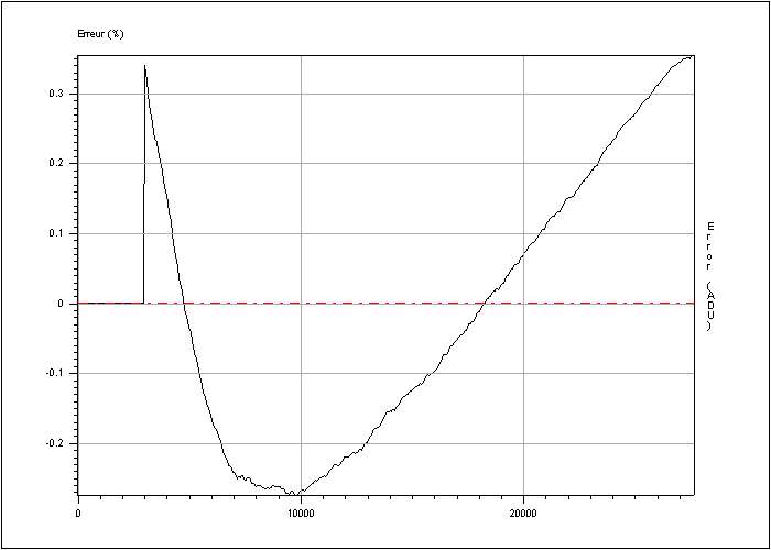
Figure 5: Error of linearity
Figure 6: Residual non linearity.
Exposure time (s) = 3600
Dark current : 0.55 ± 0 e-/hour/pixel
Cosmic event rate : 1.16 ± 0.01179 events/min/cm²
Horizontal CTE = 0.999992
Vertical CTE = 0.9999997
In this section we expose the hot pixel, the dark pixel, the trap and the very large trap we found and how.
A hot pixel provides a signal of > 60 e- / pixel / hour. To find them we use a median dark image. We take the median of the image and to find the hot point we add the mean in (e- / pixel / hour) plus the limit (60 e- / pixel / hour). All the pixel which have a value upper than this limits are considered as hot pixel. I repeat this manipulation with two other median filter to confirm the results
Result: One hot points.
On our images this point is to the coordinates:
|
Position |
Image |
Histogram around the hot pixel |
X= 0441 Y= 0948 |
|
|
Table 5: Position and images of the hot pixels.
A dark pixel is one with 50% or less than the average output for uniform intensity light level, measured with a flat field level around 500 photo-electrons.
Result: No dark pixel detected.
A trap is defined as a pixel that captures more than 10 electrons, measured with a flat field level around 500 photo-electrons.
Result: Not available
A very large trap is defined as a pixel that captures more than 10 000 electrons, measured with a flat field level around 90% of full well capability.
Result:
On our images this point is to the coordinates:
|
Position |
Image |
Histogram around the very large trap |
|---|---|---|
X= 1571; Y= 2661 X= 1572; Y= 2661 X= 1573; Y= 2661 X= 1574; Y= 2661 |
|
|
Table6: Position and images of the very large trap.
A bad column is 10 or more contiguous hot or dark pixels in a single column or a very bright pixel or a very large trap.
Result: Four bad columns. The bad columns start to the point
X= 1571; Y= 2661
X= 1572; Y= 2661
X= 1573; Y= 2661
X= 1574; Y= 2661
Here is a summary of cosmetic defects:
|
Hot pixel |
Dark pixel |
Trap |
Very large trap |
Bad column |
|---|---|---|---|---|
|
1 |
\ |
\ |
4 |
4 |
Table 7: Summary of cosmetic defects.
Back to the overview page ESO Test Reports for the OmegaCAM CCDs