Plot
? |
Symb
? |
Source
* |
Average ? |
Thresholds ? |
N_
data |
QC1
parameter |
Data
downloads |
Remarks |
| method |
value |
unit |
method |
value |
| 1 |
• | QC1DB |
MEDIAN |
8.93892 |
NONE |
VAL | 8.903,9.103 |
38 |
ArIII_r2 |
this |
last_yr |
all
|
ArIII_R2 |
| 2 |
• | QC1DB |
MEDIAN |
10.489 |
microns |
VAL | 10.444,10.644 |
38 |
SIV_r2 |
this |
last_yr |
all
|
SIV_R2 |
| 3 |
• | QC1DB |
MEDIAN |
12.75646 |
microns |
VAL | 12.696,12.896 |
38 |
NeII_r2 |
this |
last_yr |
all
|
NeII_R2 |
| 4 |
• | QC1DB |
MEDIAN |
8.93892 |
microns |
VAL | 8.835,9.035 |
38 |
ArIII_r3 |
this |
last_yr |
all
|
ArIII_R3 |
| 5 |
• | QC1DB |
MEDIAN |
10.489 |
microns |
VAL | 10.446,10.646 |
38 |
SIV_r3 |
this |
last_yr |
all
|
SIV_R3 |
| 6 |
• | QC1DB |
MEDIAN |
12.75646 |
microns |
VAL | 12.66,12.86 |
38 |
NeII_r3 |
this |
last_yr |
all
|
NeII_R3 |
| 7 |
• | QC1DB |
MEDIAN |
9.00272 |
microns |
VAL | 9.0,9.05 |
37 |
ArIII_r2 |
this |
last_yr |
all
|
ArIII_R2 |
| 8 |
• | QC1DB |
MEDIAN |
10.46631 |
microns |
VAL | 10.442,10.492 |
37 |
SIV_r2 |
this |
last_yr |
all
|
SIV_R2 |
| 9 |
• | QC1DB |
MEDIAN |
12.8176 |
microns |
VAL | 12.793,12.843 |
37 |
NeII_r2 |
this |
last_yr |
all
|
NeII_R2 |
| 10 |
• | QC1DB |
MEDIAN |
9.04693 |
microns |
VAL | 9.023,9.073 |
37 |
ArIII_r3 |
this |
last_yr |
all
|
ArIII_R3 |
| 11 |
• | QC1DB |
MEDIAN |
10.46674 |
microns |
VAL | 10.464,10.514 |
37 |
SIV_r3 |
this |
last_yr |
all
|
SIV_R3 |
| 12 |
• | QC1DB |
MEDIAN |
12.81802 |
microns |
VAL | 12.815,12.865 |
37 |
NeII_r3 |
this |
last_yr |
all
|
NeII_R3 |
| |
|
*Data sources: QC1DB: QC1 database; LOCAL: local text file
|
| Plot 1 | | data source: | midi_wave
(QC1 database) |
| dataset: | ArIII_r2 | • |
| median: | 8.93892 | NONE |
| fixed thresholds: | 8.903...9.103 | NONE |
| N_data plotted: | 38 |
| [click on plot for closeup] |
| Plot 2 | | data source: | midi_wave
(QC1 database) |
| dataset: | SIV_r2 | • |
| median: | 10.489 | microns |
| fixed thresholds: | 10.444...10.644 | microns |
| N_data plotted: | 38 |
| [click on plot for closeup] |
| Plot 3 | | data source: | midi_wave
(QC1 database) |
| dataset: | NeII_r2 | • |
| median: | 12.75646 | microns |
| fixed thresholds: | 12.696...12.896 | microns |
| N_data plotted: | 38 |
| [click on plot for closeup] |
| Plot 4 | | data source: | midi_wave
(QC1 database) |
| dataset: | ArIII_r3 | • |
| median: | 8.93892 | microns |
| fixed thresholds: | 8.835...9.035 | microns |
| N_data plotted: | 38 |
| [click on plot for closeup] |
| Plot 5 | | data source: | midi_wave
(QC1 database) |
| dataset: | SIV_r3 | • |
| median: | 10.489 | microns |
| fixed thresholds: | 10.446...10.646 | microns |
| N_data plotted: | 38 |
| [click on plot for closeup] |
| Plot 6 | | data source: | midi_wave
(QC1 database) |
| dataset: | NeII_r3 | • |
| median: | 12.75646 | microns |
| fixed thresholds: | 12.66...12.86 | microns |
| N_data plotted: | 38 |
| [click on plot for closeup] |
| Plot 7 | | data source: | midi_wave
(QC1 database) |
| dataset: | ArIII_r2 | • |
| median: | 9.00272 | microns |
| fixed thresholds: | 9.0...9.05 | microns |
| N_data plotted: | 37 |
| [click on plot for closeup] |
| Plot 8 | | data source: | midi_wave
(QC1 database) |
| dataset: | SIV_r2 | • |
| median: | 10.46631 | microns |
| fixed thresholds: | 10.442...10.492 | microns |
| N_data plotted: | 37 |
| [click on plot for closeup] |
| Plot 9 | | data source: | midi_wave
(QC1 database) |
| dataset: | NeII_r2 | • |
| median: | 12.8176 | microns |
| fixed thresholds: | 12.793...12.843 | microns |
| N_data plotted: | 37 |
| [click on plot for closeup] |
| Plot 10 | | data source: | midi_wave
(QC1 database) |
| dataset: | ArIII_r3 | • |
| median: | 9.04693 | microns |
| fixed thresholds: | 9.023...9.073 | microns |
| N_data plotted: | 37 |
| [click on plot for closeup] |
| Plot 11 | | data source: | midi_wave
(QC1 database) |
| dataset: | SIV_r3 | • |
| median: | 10.46674 | microns |
| fixed thresholds: | 10.464...10.514 | microns |
| N_data plotted: | 37 |
| [click on plot for closeup] |
| Plot 12 | | data source: | midi_wave
(QC1 database) |
| dataset: | NeII_r3 | • |
| median: | 12.81802 | microns |
| fixed thresholds: | 12.815...12.865 | microns |
| N_data plotted: | 37 |
| [click on plot for closeup] |
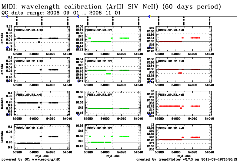
The wavelength day calibration consists in using the MIDI heated
blackscreen and taking 3 exposures through different narrow-band
filters [NeII], [SIV] and [ArIII] (having central wavelengths
accurately measured in the laboratory by the manufacturer). An extra
exposure is taken through a polycarbonic foil that has several
absorption lines in its N-band spectrum. Exposures without filters and
with closed shutter are also taken to process the exposures with
filters. From the spectra obtained through the filters a fit of the
lambda(X) function is performed. The procedure is performed for each
setup (PRISM or GRISM, and SCI_PHOT or HIGH_SENS). The MIDI HIGH_SENS mode
uses 2 windows on the detector (R1 and R2). The MIDI SCI_PHOT mode uses 4
windows (R1 to R4)
We monitor here the stability of the dispersion by plotting the
wavelength of a spectral channel given by the lambda(X) function
computed by the reduction of the calibration data. The selected
spectral channels corresponds to the expected central wavelength of the
three narrow-band filters.
General information
Click on any of the plots to see a close-up version.
The latest date is indicated on top of the plot, data points belonging to that date are specially marked.
If configured,
- statistical averages are indicated by a solid line, and thresholds by broken lines
- outliers are marked by a red asterisk. They are defined as data points outside the
threshold lines
- "aliens" (= data points outside the plot Y limits) are marked by a red arrow (↑ or ↓)
- you can download the data for each parameter set if the 'Data downloads' link shows up
|
