The Tololo SLODAR Campaign
(November 24-December 3,
2004 )
Final Report,
Marc Sarazina, Tim Butterleyc, Andrei Tokovininb, Tony Travouillond,
Richard
Wilsonc
a- European Southern Observatory (ESO), b- Cerro Tololo Inter-American Observatory (CTIO),
c-

Table of Contents
The Tololo SLODAR Campaign...................................................................................... 1
Table of Contents............................................................................................................. 2
Introduction..................................................................................................................... 3
1- Instruments Description................................................................................................ 4
1. a- Acoustic Sounder: SODAR................................................................................. 4
1.b- Wave front Monitor: SLODAR............................................................................. 5
1.c- Scintillation Sensor: MASS................................................................................... 8
1.d- Differential Image Motion Monitor: DIMM.......................................................... 10
2- Night Summaries....................................................................................................... 11
2.a- Explanation of the plots....................................................................................... 11
2.b- Night 24-25 November...................................................................................... 12
2.c- Night 25-26 November...................................................................................... 13
2.d- Night 26-27 November...................................................................................... 14
2.e- Night 27-28 November...................................................................................... 15
2.f- Night 28-29 November....................................................................................... 16
2.g- Night 30 November-01 December...................................................................... 17
2.h- Night 01-02 December....................................................................................... 18
2.j- Logbook............................................................................................................. 19
3- Local Meteorology.................................................................................................... 21
4- Instrument Comparison.............................................................................................. 24
4.a- SLODAR and DIMM integrals, all data.............................................................. 24
4.b- SLODAR and MASS-DIMM integrals, all data.................................................. 25
4.c- SODAR and MASS-DIMM integrals, all data.................................................... 28
4.d- SLODAR-WB & SODAR GL binned profiles for selected time
intervals............ 29
5- Discussion................................................................................................................. 34
Appendix....................................................................................................................... 35
A.a- Database Description......................................................................................... 35
A.b- List of available SLODAR targets...................................................................... 36
Introduction
A 2-week campaign comparing vertical turbulence profile
monitoring instruments took place from November 24 to
The purpose is to compare currently available techniques for monitoring the effective thickness of the ground layer turbulence in the framework of the feasibility study of Ground-Layer Adaptive Optics (GLAO). In the AO terminology, ground layer (GL) refers to the lower part of the turbulence profile which could be corrected by a single deformable mirror over a wide field of view. Note that this definition includes the part of the atmosphere dominated the local ground effects (first 100m) and extends into the atmospheric boundary layer (first 1000m or more) influenced by larger scale orographic features.
Figure 1: Field layout of the instrumentation on the eastern side of the Tololo platform (from left to right): SODAR, USNO (control room), CTIO MASS-DIMM tower, SLODAR, CELT T3 MASS-DIMM tower
Three methods are compared in this campaign for GL monitoring:
-Acoustic sounding: a SODAR delivers high vertical resolution (20m) profiles of back-scattered acoustic energy in the first half-kilometer. A specific calibration is necessary for conversion into index of refraction structure coefficient (Cn2)
-Wave front slope monitoring: SLODAR
(SLOpe Detection And Ranging) delivers medium (150m) or
low (1500m) resolution Cn2 profiles when appropriate binary stars are
available.
-Difference of integral seeing measured by DIMM and high layers seeing measured by MASS. DIMM-MASS is a fair representation of the total turbulence in the GL for GLAO applications.
1- Instruments Description
1.a- Acoustic Sounder: SODAR
An acoustic sounder, SODAR (model XFAS from Scintec, http://www.scintec.com) has been installed by CTIO. The location is selected to avoid as much as possible, fixed echoes from the nearby USNO but close enough to the DIMM-MASS T3 tower and the SLODAR. The SODAR antenna is protected from the ambient noise during reception by absorbing walls which also reduce ambient noise contamination during emission
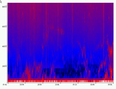
Figure 2: Example of SODARgram starting
Critical Data Analysis:
The deficiency of the SODAR used in this campaign is its lower altitude limit of 40m. Thus, an important part of the strong turbulence in the first meters above the ground was not sensed, complicating direct comparisons with other instruments. The SODAR sensitivity at altitudes above ~400m was affected by ambient noise originating from nearby domes, vents are cooling systems of the observatory (variable noise level), on some heights a strange pattern in the Doppler images suggests a constant source of noise probably caused by the vents of the 4m telescope occasionally oriented toward the SODAR. The noise pollution was partially reduced by software. The calibration of SODAR does not take into account humidity variations that might affect high-altitude return signal. The relative humidity variation during observations was from 5% to ~60%. The calibration used is valid for humidity around 20%, so SODAR data on Nov. 24 and 25 are not expected to be accurate. The SODAR sees a lot more turbulence below 100m than the SLODAR. It could be the SODAR calibration which is not yet perfect, for example sometimes missing the first point of data. Comparing the seeing values with MASS_DIMM as in Figure 24, it also shows that when the seeing is really bad the SODAR overestimates it. This is something which needs to be thought about (non-linearity of calibration?).
1.b- Wave front Monitor: SLODAR
A prototype portable seeing and
turbulence monitor based on the SLODAR method was developed for ESO by R.
Wilson from the AIG Durham (http://aig-www.dur.ac.uk/fix/projects/slodar/). The
system comprises a Meade 40cm telescope equipped with an 8x8 element Shack-Hartmann
WFS (5cm sub-apertures). The turbulence altitude profile is recovered from the
time-averaged spatio-angular cross-correlation of the
instantaneous wave front slopes, measured in the telescope pupil plane by using
a Shack-Hartmann wave front sensor to observe a bright binary star. A vertical
resolution of about 1.5km could be achieved for observations of narrow (5-7”)
binary stars (SLODAR-NB) and down to 150m when observing wide binaries
(55-60”). Exposure times of the order 1-2 milliseconds are required in order to
'freeze' the seeing-induced motions of the WFS spots on 5cm apertures, placing
strict requirements on the detector system. In order to achieve continuous monitoring,
a limiting magnitude of V~7 for individual binary components is required
to provide sufficient target stars. A detector with high QE, and read-out noise
less than 1 electron rms is necessary. A camera based
on the new E2V L3Vision CCD technology (http://e2vtechnologies.com/introduction/prod_l3vision.htm),
such as the Andor Technology iXon
CCD cameras (http://www.andor-tech.com/),
meet these requirements.
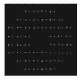
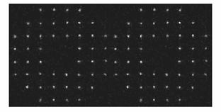
Figure 3: SLODAR Shack-Hartman pattern using narrow (left) and wide (right) binaries.
In Figure 3, the binary star projects ‘copies’ of the wave front
aberration produced by the turbulent layer at altitude H onto the ground, with
separation S. Hence there is a peak in the slope cross-correlation function for
spatial offset S. H can be found by triangulation, given the binary star
separation angle (theta). The strength of the layer is related to the amplitude
of the cross-correlation signal (Figure
5). The full normalized profile is recovered from the
cross-correlation via a de-convolution, where the autocorrelation of the wave
front slopes for a single star of the binary is used as a measure of the
(altitude-independent) impulse response of the system to a single turbulent
layer. Although the cross-correlation is in two dimensions, we need only
consider a cut through the function in the direction of the binary star
separation. The total integrated turbulence, quantified by Fried’s
parameter r0, is found from the variances of the Zernike
aberration terms for the centroid data (Figure 4).
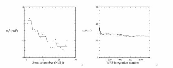
Figure 4: An example SLODAR determination of
r0. Left: Measured Zernike coefficient variances, σj (crosses) and the theoretical (Noll) fit (solid
line). Right: Calculated value of r0 versus WFS integration number (2ms CCD
integrations at 190Hz)
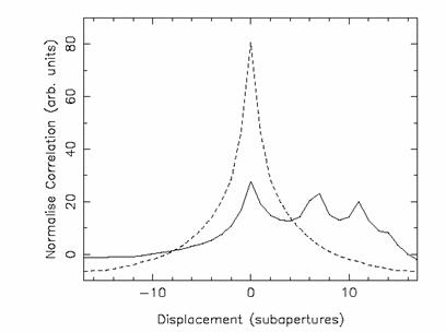
Figure 5: 1-D simulated cross-correlation (solid line) and autocorrelation (broken line) in the direction of the binary separation for a 24x24 sub-aperture.
Critical Data
Analysis:
a) The altitude resolution of SLODAR depends on the separation of the selected binary and on the zenith angle. Thus for a given target, the altitudes of "layers" change with time, following the cos(z) law.
b) Strong scintillation reduces the measured centroid variance, resulting in over-estimation of r0.
Hence the PPS under-estimates r0 when there is strong high altitude turbulence,
and/or when the airmass is large. Further investigation is required
to establish whether this is a fundamental physical effect, or whether the
current centroider algorithm begins to fail in strong
scintillation (or both). Increasing scintillation is the most likely
cause of the trend with airmass. Also, most of the narrow binary data was
by chance taken in conditions where much of the turbulence was high, or in high
airmass. So it is perhaps not clear that there is a specific problem
with the narrow binary mode cf. the wide mode. In the case of Figure 33 there was strong scintillation and SLODAR significantly
underestimated the total Cn2, so that the entire SLODAR curve is too low.
c) SLODAR deconvolution is producing in some cases a negative offset in the second resolution element (first above the ground):
This results from deconvolving with a PSF which is not appropriate for the 'zero' altitude layer: for Kolmogorov turbulence, tilts between neighboring sub-apertures are approx. 40% correlated. But the cross correlation signal from turbulence in the first element (<100m) shows much lower correlation (often close to zero) between neighboring sub-apertures, presumably due to a very short outer scale. Currently we de-convolve using an impulse response which is the auto-correlation measured using the whole Cn2 profile, including higher layers with (presumably) much larger outer scales (a few tens of meters, at least). The result is a negative bias at +1 and -1 sub-apertures offset. Typically the negative offset is 20 to 30% of the signal in the first (0km) element.
For example in Figure 30: SODAR gives a strong signal at ~ 150m, whereas SLODAR is actually negative (-1e-16). SLODAR 0km strength is 12e-16, so if we add 0.3*12e-16 = 4e-16, we get 3e-16 in the 160m SLODAR bin. This then agrees with SODAR, when SODAR is averaged over 80-240m. Treated in this way, most of the SLODAR-SODAR plots would agree better in the region of the second SLODAR resolution element (~80-230m).
It is perhaps surprising that the
very low level turbulence should have such a very small outer scale (i.e. to
reduce the correlation between neighboring 5cm sub-apertures) -although we
might expect any dome/mirror seeing to produce this effect.
The key question is how to deal with the effect in the analysis. The de-convolution
error also produces a spurious negative value in the first resolution element
of the profile at NEGATIVE altitude, which should have value zero. Hence we can
use this value to estimate and correct for the de-convolution error.
Bibliography:
-Wilson R.W., “SLODAR: Measuring optical turbulence altitude with a Shack--Hartmann wave-front sensor”, MNRAS 337, 103, 2002.
-Wilson, R.W & Saunter, C.D., “Turbulence profiler and seeing monitor for laser guide star adaptive optics”, proc. SPIE 4839, 446, 2003.
1.c- Scintillation Sensor: MASS
MASS (Multi Aperture Scintillation Sensor) is a small instrument to measure vertical turbulence profile (http://www.ctio.noao.edu/~atokovin/profiler/). Unlike previous techniques, it is simple and inexpensive, destined to work continuously as a turbulence monitor at existing and new sites. MASS is based on a statistical analysis of stellar scintillations in four concentric ring apertures.
Figure 6: MASS principle, scintillation of a single star
is measured through 4 concentric annular apertures.
This novel approach was proposed
in 1998 and tested the same year at
The vertical resolution of MASS
is low, only about 1/2 of altitude. The whole atmosphere is subdivided into 6
thick slabs (.5, 1, 2, 4, 8 and 16km) and the turbulence intensity in each
layer is measured. Ground-layer turbulence does not produce any scintillation;
it is not sensed by MASS. On the other hand, DIMM senses the whole atmosphere.
Turbulence intensity in the ground layer can be found by combining MASS and
DIMM data: the two instruments should always work together. For that purpose a
combined MASS-DIMM pupil segmentator was developed where
the same telescope feeds both instruments: two apertures are sent to the DIMM
channel whereas four concentric apertures are cut to feed the MASS detectors.
Critical Data Analysis:
The integral characteristics of turbulence are measured by MASS quite reliably. However, the profile restoration is delicate; hence sometimes turbulence is attributed to wrong layers. The restoration errors are largest in the lowest (0.5km) layer, most important for this campaign.
MASS restoration is based on linear theory applicable to very weak scintillation. It was found that MASS systematically over-estimates the turbulence integral ("overshoots") when the scintillation index exceeds ~0.1. A first-order correction to overshoots, found by numerical simulations, is applied to the MASS data of this campaign. However, in some cases (notably for fast turbulence) some residual over-shoots may remain. In this case the ground-layer turbulence estimated from DIMM minus MASS is under-estimated.
Bibliography:
-Kornilov
V.G., Tokovinin A.A. Measurement of the turbulence in
the free atmosphere above
-Tokovinin
A., Kornilov V., Shatsky
N., Voziakova O. Restoration of turbulence profile
from scintillation indices. MNRAS, 2003, V.
343, p. 891-899 [PDF, 419K ]
1.d- Differential Image Motion Monitor: DIMM
The DIMM optical system developed for the CELT site testing campaign (http://galaxy.ps.uci.edu/%7Eceltsite/equipment.html) is based on the MASS-DIMM optics of section 1.c that splits the pupil by mirrors. MASS and DIMM use the same telescope and same star, hence sample common turbulent volume. All other instruments do not share this feature.
The CCD detector used in the CELT DIMM system is an SBIG ST7 (http://www.sbig.com/). The innovative feature of the CELT DIMM system is the manner in which the DIMM data is taken. Normal DIMM systems generally take interlaced 5ms and 10ms exposures with a dead time of the approximately 200ms between each exposure. However the CELT DIMM system utilizes a continuous or drift mode readout facility that allows exposures as short as 3.5ms with negligible dead time between exposures. So rather than a sequence of interlaced short exposure images separated by large dead time, we obtain a continuous sequence of very short exposures. The continuous sequence of images that we obtain allows for more sophisticated analysis techniques. In-software binning in the readout direction gives us effective exposure times of any length. Thus we can improve on the simpler two exposure time technique of Tokovinin 2002 for determining the seeing at zero exposure time by fitting an exponential function to the seeing measured in a range of time bins.
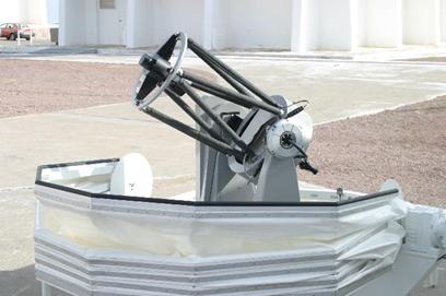
Figure 7: The TMT DIMM telescope is a 35cm
Cassegrain in an alt-az
mount produced by Halfmann Teleskoptechnik
in
Critical Data Analysis:
Optical aberrations of DIMM feeding optics bias the measured seeing to higher values. This effect was confirmed during intensive comparisons of two identical MASS-DIMM units. After careful control of the optical quality was implemented, the instruments agreed to within 0.02". The optics of T3 used in this campaign was monitored by recording Strehl ratios, thus the DIMM data are not biased.
Bibliography:
Tokovinin
A., From differential image motion to seeing. PASP, 2002, V. 114, P. 1156 [PDF, 179K ]
2- Night Summaries
2.a-
Explanation of the plots
Explanation of the plots in Figure 8 to Figure 14
1-Upper
left quadrant:
The SODAR (top) and SLODAR (bottom) turbulence profiles are displayed in the square-root as a function of UT (vertical tics, 1h spacing). The lowest SODAR level is at 40m, followed by 40 layers of 20m thickness. The horizontal line marks the 400m level. A turbulence profile is obtained every 20 min. In wide binary (WB) mode, SLODAR monitors the GL from ground level up to typically 1000m in 150m steps depending on binary angular separation and airmass. The horizontal line marks the 500m level.
2-Upper
right quadrant:
The integrated seeing in the ground layer, in the 0.5-km layer and above from MASS-DIMM (line), SLODAR (asterisks) and SODAR (dashes) are compared, with a temporal binning of 12min (0.2h) for each night. The three sub-layers correspond to the estimated coverage of, respectively, DIMM minus MASS integral, MASS 0.5km and the sum of the 5 MASS upper layers (fixed layers mode).The respective weighting functions used to build the SLODAR vertical bins are plotted in Figure 21. Note that the upper layer of SLODAR includes the “un-sensed” Cn2 which is the difference between the SLODAR integral and the sum of the 8 SLODAR layers. SODAR integrals in the GL were computed with a weight that is 1 from 40 to 250m, and then drops linearly to zero at 500m.
3-Lower left
quadrant
Mass profiles in the fixed layer mode: the bar-plots of Cn2
integral in 6 pre-defined layers as a function of UT time. The length of bars is
proportional to the Cn2 integral in each layer. The scale
corresponds to 5E-13m1/3 for a vertical bar length equal to the
distance between layers.
4-Lower right
quadrant
Similarly to DIMM, MASS and SLODAR also produce an estimate
of the integrated seeing independently of the profile reconstruction. However,
MASS integral (red line) neglects the first 500m of atmosphere which does not
produce scintillation. On the other hand, SLODAR is expected to produce, both
in wide (blue dots) and narrow (green dots) binary mode, a seeing integral over
the whole light path after removal of dome/telescope contribution. As SLODAR is
at ground level, it should find slightly higher values than DIMM which is at 7m
above ground.
2.b- Night 24-25
November
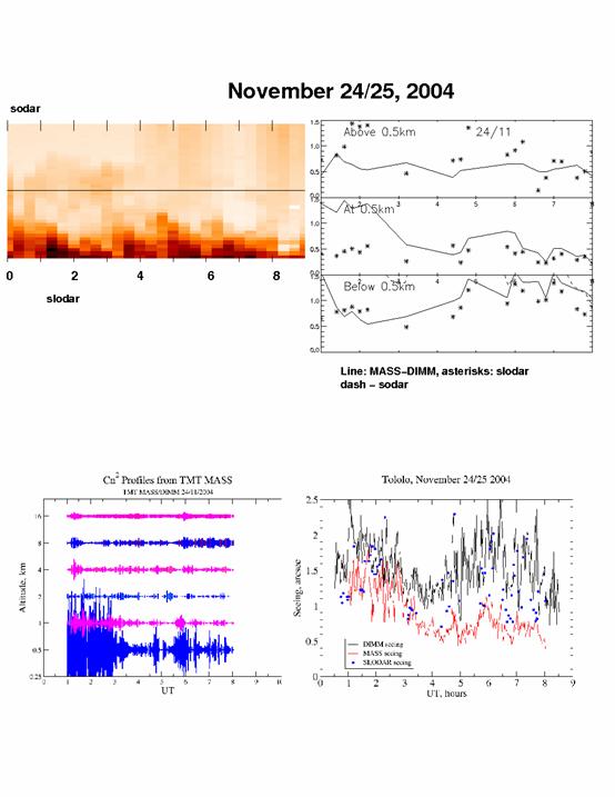
Figure 8: Summary of the data collected during
the night 24 to 25 November, 2004: see section 2.a- Explanation of the plots. Note here that the SODAR line spills beyond
the plot boundary in the upper right quadrant,
2.c- Night
25-26 November
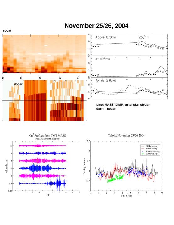
Figure 9: Summary of the data collected during the night
25 to 26 November, 2004: see section 2.a- Explanation of the plots
2.d- Night
26-27 November

Figure 10: Summary of the data collected during the night 26 to 27 November, 2004: see section 2.a- Explanation of the plots.
2.e-
Night 27-28 November
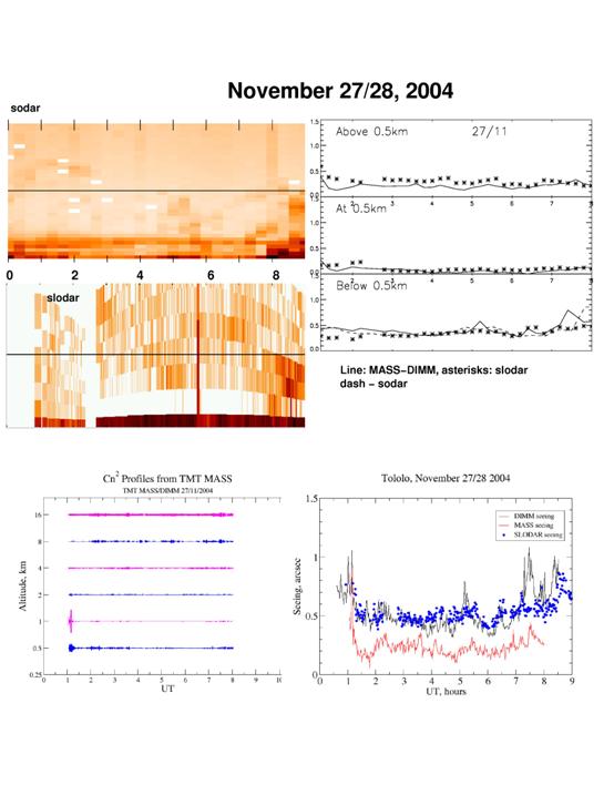
Figure 11: Summary of the data collected
during the night 27 to 28 November, 2004: see section 2.a- Explanation of the plots.
2.f-
Night 28-29 November
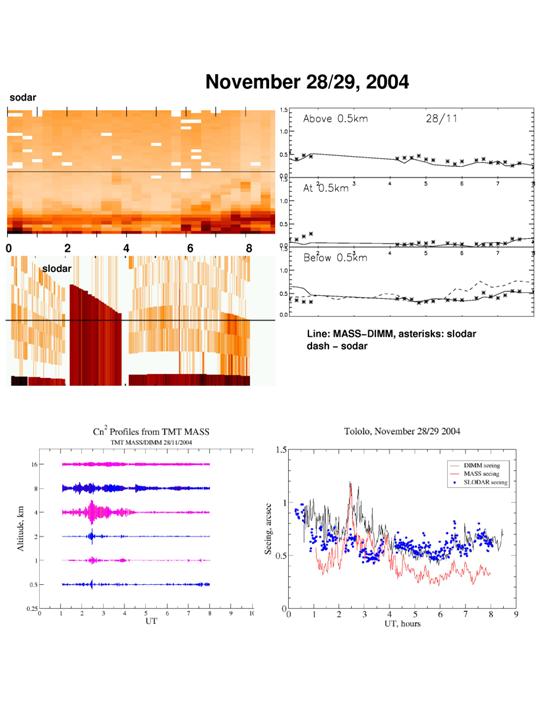
Figure 12: Summary of the data collected during the night 28 to 29 November, 2004: see section 2.a- Explanation of the plots.
2.g-
Night 30 November-01 December
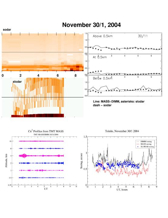
Figure 13: Summary of the data collected
during the night 30 November to
2.h-
Night 01-02 December
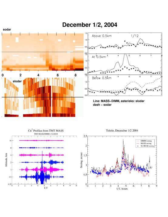
Figure 14: Summary of the data collected during the night 01 to 02 December, 2004: see section 2.a- Explanation of the plots.
2.j- Logbook
Arrival at La Serena of
Richard Wilson & Tim Butterley
19,20 November, SLODAR
unpacking and assembly
Night 21-22 November
Clear, first SLODAR data
taken, seeing 1.0-1.2-0.8"
Night 22-23 November
Seeing 1.5-1",
improving at the end of night
Reshuffle SLODAR power supply
scheme (110-220V converter needed for CELT). Relay box not working afterwards
due to bad contact. High absorption, few data were taken.
Night 23-24 November
Colder temperature, overcast
until 5hUT, no useful data taken afterwards either. Review of SLODAR principle
with A. Tokovinin.
Night 24-25 November
Clear sky, Wind 5-10m/s
The SLODAR data reduction algorithm
cannot track spots when the S-H pattern hits the image sides, this can be
improved (2ms exposure should freeze any wind shake).Bad seeing conditions
2" to 1.5" all night very variable, 80% in the first km.
Night 25-26 November
Clear sky, low wind, seeing
1"
Time lost for various
crashes of the SLODAR data processing GUI, restart somewhat laborious because
accumulated incoming files have to be moved manually before re-start. Auto-guiding
not working properly
-Very stable conditions at
beginning of night, 1" seeing, most of it above 1km, 57" wide binary
from 00h30 to 01h30, agreement with SODAR (no turbulence).
-Change to 6.8" narrow
binary (one much brighter). Exchange of SH lenslet
array: refocus procedure very slow because focus remote control is not working
since the day before (hardware).
SLODAR underestimates total
seeing but shows dip at 1km and peak above 2km (the value of r0 displayed does
not agree with the value plotted). MASS is overshooting, 2km layer pulsating,
seeing stable at 1".
-Change to 53" wide
binary. SODAR shows low level turbulence rising, OK with SLODAR although the
share of the low level turbulence is only 20% of Cn2 at 1" seeing.
Dominating contribution comes from the higher atmosphere (80% of Cn2).
Night 26-27 November
Clear sky, low wind, seeing
0.5", long tau0 (W200mb=20m/s), no ground level (SODAR) turbulence, thus
we shall work with narrow binaries.
New CCD control GUI
implemented (thanks Tim!), considerably less overhead, auto-guiding working.
Next improvement is automated data acquisition. Focus drive still not working.
-5.5" narrow binary
(both faints) to check r0 discrepancy: better agreement tonight with T3 DIMM
but still larger r0. Good agreement with MASS: .6 to 1.0 10^-13 above 8km.
Lower turbulence at 2km seen by both instruments at 02h20UT. SLODAR definitely
underestimating seeing, r0 seems to get larger with increasing airmass!!
Automated acquisition mode
implemented, the data rate ia about one per minute,
life is now much better.
-53" wide binary, at
5h30 UT, the centroiding threshold is changed
manually and SLODAR agrees well with DIMM T3. High atmosphere absolutely clean
(0.2"), SODAR sees no turbulence either, hence the bulk of the turbulence
(0.5") should now be in the first 50m.
Night 27-28 November
Seeing 0.5”, low wind.
SLODAR: All night wide
binary. First target until UT=2.2656 was faint, noise is underestimated, hence
high layer over-estimated. Remainder of night is bright target (trapezium), so
better agreement with MASS free atmosphere.
But SLODAR r0 < DIMM r0 for much of the night - dome seeing or
<20m contribution? (all extra Cn2 in first pixel?). Appearance of layer at
~300-400m at end of night was mirrored by SODAR.
Night 28-29 November
Seeing
0.5-1.1”, low wind.
SLODAR begins
with wide binary, then close binary for ~
Night 28-29 November: break
Night 30 November – 01 December
The
night of Tuesday was clear, with a good seeing and "empty" ground
layer (excepted the lowest) - i.e. "boring". We stopped at ~4h local
as people were tired. Tony looked at the SODAR, we discovered some problems
with response at high layers.
Night 01-02 December
Descending
turbulent layer, becoming more 'aggressive'
as it nears the ground, then apparently fading and 'rebounding' upward?
Separate image thresholds for the centroiding of the
two stars, were introduced in the SLODAR reduction software to avoid problems
where the magnitude difference was significant.
3- Local Meteorology
 Figure
15: Local air temperature in
Celsius during the Tololo SLODAR Campaign.
Figure
15: Local air temperature in
Celsius during the Tololo SLODAR Campaign.
 Figure
16: Local relative humidity in
percent during the Tololo SLODAR Campaign.
Figure
16: Local relative humidity in
percent during the Tololo SLODAR Campaign.
 Figure
17: Local wind speed (m/s)
during the Tololo SLODAR Campaign
Figure
17: Local wind speed (m/s)
during the Tololo SLODAR Campaign
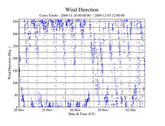 Figure
18: Local wind direction in
degree (0=North, 90=East) during the Tololo SLODAR
campaign.
Figure
18: Local wind direction in
degree (0=North, 90=East) during the Tololo SLODAR
campaign.
 Figure
19: Local air pressure (mB) during the Tololo SLODAR
Campaign
Figure
19: Local air pressure (mB) during the Tololo SLODAR
Campaign
4- Instrument Comparison
4.a- SLODAR and DIMM integrals, all data
The seeing values in the whole atmosphere measured by DIMM and SLODAR are compared, with a temporal binning of 12min (0.2h) on Figure 20. Seeing is corrected at zenith and computed for 0.5 micron wavelength. As shown in Figure 1, SLODAR is at ground level while DIMM is on a 6m high tower. This height difference explains the excess seeing measured by SLODAR in excellent seeing conditions. Otherwise SLODAR shows a linear underestimation of the seeing most likely due to an inaccurate plate scale value.

Figure 20: Comparison of DIMM (8m above ground) and SLODAR (ground level, WB mode) simultaneous estimates of the turbulence in the whole atmosphere (12mn bins).
4.b- SLODAR and MASS-DIMM integrals, all data
The integrals in the ground layer, in the 0.5-km layer and above from MASS-DIMM and SLODAR are compared, with a temporal binning of 12min (0.2h). The three sub-layers correspond to the estimated coverage of, respectively, DIMM minus MASS integral, MASS 0,5km and the sum of 5 MASS upper layers (fixed layers mode).The respective weighting functions used to convert SLODAR into MASS-DIMM vertical bins are plotted in Figure 21. Note that the upper layer of SLODAR includes the “unsensed” Cn2 which is the difference between the SLODAR integral and the sum of the 8 SLODAR layers.

Figure 21: Weighting functions for merging SLODAR profiles into MASS-DIMM integral footprints: lower ground layer (full line), 500m layer (dashes) and whole atmosphere above 0.5km (dots).
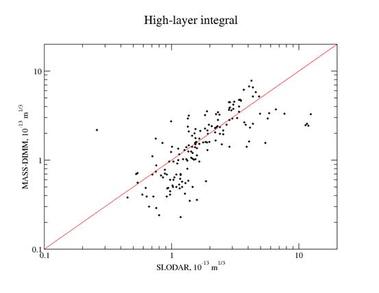
Figure 22: Comparison of MASS-DIMM and SLODAR simultaneous estimates of the turbulence above 0.5km (12mn bins).

Figure 23: Comparison of MASS-DIMM and SLODAR simultaneous estimates of the 500m layer turbulence (12mn bins).

Figure 24: Comparison of MASS-DIMM and SLODAR simultaneous estimates of the lower GL turbulence (12mn bins).
4.c- SODAR and MASS-DIMM integrals, all data
The XY comparison of simultaneous integrals of GL seeing measured by MASS-DIMM and SODAR during our campaign is shown on Figure 25. The SODAR was weighted in altitude with a weight 1 up to 250m, then a linear fall to 500m. MASS-DIMM was averaged during SODAR 20-min. integrations, with a minimum of 4 MASS-DIMM points required. The MASS "overshoots" are, of course, corrected. The night of Nov. 24 is excluded (high humidity).
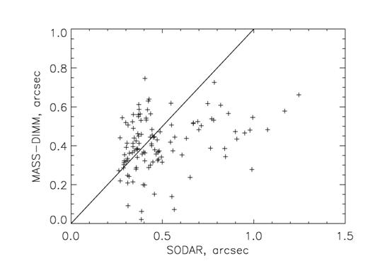
Figure 25: Comparison of MASS-DIMM and SODAR
simultaneous estimates of the lower GL turbulence (12mn bins).
4.d- SLODAR-WB & SODAR GL binned profiles for selected time intervals
Here, we select the SODAR profiles corresponding to a given time interval MM minutes, i.e. labeled between hh:mm and hh:mm+MM. Given that the SODAR profiles are labeled by the end of the 20mn accumulation time, the actual duration of the synchronous time-averaged SLODAR interval is MM+20 min. The following plots show clearly the effect of the difference in the altitude resolution of the two instruments: ~160m for SLODAR versus 20m for SODAR. Hence narrow spikes visible in the SODAR profiles will not be resolved in the SLODAR profiles.

Figure 26: Vertical profile of the turbulence
in the GL as monitored by SLODAR (full line) and SODAR (dashes) on

Figure 27: Vertical profile of the
turbulence in the GL as monitored by SLODAR (full line) and SODAR (dashes) on

Figure 28: Vertical profile of the turbulence
in the GL as monitored by SLODAR (full line) and SODAR (dashes) on

Figure 29: Vertical profile of the
turbulence in the GL as monitored by SLODAR (full line) and SODAR (dashes) on

Figure 30: Vertical profile of the turbulence
in the GL as monitored by SLODAR (full line) and SODAR (dashes) on November 30-
 Figure
31: Vertical profile of the
turbulence in the GL as monitored by SLODAR (full line) and SODAR (dashes) on
Figure
31: Vertical profile of the
turbulence in the GL as monitored by SLODAR (full line) and SODAR (dashes) on
 Figure
32: Vertical profile of the
turbulence in the GL as monitored by SLODAR (full line) and SODAR (dashes) on
Figure
32: Vertical profile of the
turbulence in the GL as monitored by SLODAR (full line) and SODAR (dashes) on

Figure 33: Vertical
profile of the turbulence in the GL as monitored by SLODAR (full line) and
SODAR (dashes) on
 Figure
34: Vertical profile of the
turbulence in the GL as monitored by SLODAR (full line) and SODAR (dashes) on
Figure
34: Vertical profile of the
turbulence in the GL as monitored by SLODAR (full line) and SODAR (dashes) on
5- Discussion
This campaign has clearly demonstrated
that an accurate profiling of the atmospheric index of refraction structure
coefficient in the first kilometer is within reach. As a proof is the excellent
agreement between SLODAR and MASS-DIMM integrals on both ground and high layers
(Figure
22 to Figure
24).
The strengths and weaknesses of the three methods involved are listed below, keeping in mind that processing algorithms are still evolving.
|
Instrument |
Vertical Resolution |
Temporal Resolution |
Accuracy |
Sensitivity |
|
MASS-DIMM |
low |
high |
average |
high |
|
SLODAR |
average |
high |
high |
high |
|
SODAR |
high |
low |
low |
low |
The SODAR seems to see only strong turbulence, but is then able to accurately track its altitude variations with a high vertical resolution. SODAR has no sensitivity below 40m and above ~ 600m, although it would improve at a quieter site. The accuracy in terms of Cn2 is yet to be demonstrated and work is currently underway to make the calibration more accurate and humidity independent.
The MASS-DIMM has a high sensitivity of the GL turbulence thanks to the DIMM function. However the profiling accuracy is low due to the increased MASS profile inversion uncertainty in the lower layers. MASS seems to exaggerate the 0.5-km layer when it is turbulent (Figure 23). The same tendency was observed in an earlier comparison with a SCIDAR.
The SLODAR appears as the most promising instrument for the monitoring of the ground layer. However the expected high profiling accuracy can be reached only after an improvement the current software, in particular with regards to the following points:
- Under-estimation of overall seeing by SLODAR, especially with narrow binary. Because it is used to normalize the profile, if r0 is in error, it means the same error is transmitted to the profile. The overall seeing is under-estimated if there is strong scintillation (strong high layers and/or high airmass). Further investigation is required to establish (a) whether this is purely a physical effect or whether there are centroider issues involved, (b) how to use scintillation measures (intensity fluctuations of the WFS spots) to re-calibrate the profile correctly (in the case that it is purely a physical effect), and (c) the accurate plate scale value of the wave front sensor.
- Dependence of the derived seeing on the centroiding parameters (threshold) and binary magnitudes.
- Trends of SLODAR seeing with air mass (despite correction) are probably due to the scintillation bias, but need to confirm this quantitatively.
- De-convolution issues, in particular producing a negative bias in the first resolution element above the ground, when there is significant turbulence with very small outer scale in the lowest layer (e.g. mirror or dome seeing). This effect should be corrected by using the first negative altitude point in the centroid cross-correlation.
Appendix
A.a- Database Description
The following instruments are included in the Tololo SLODAR campaign, with the respective responsible for
data processing:
-SLODAR, Richard Wilson,
-SODAR, Tony Travouillon, Caltech
-MASS-T3, Andrei Tokovinin, CTIO
-DIMM-T3, Andrei Tokovinin, CTIO
-Meteo Mast, Tololo
Each instrument provides data files with the format
described below. The data files contain only valid data after reduction.
1- SLODAR
UTDATE (YYYY MM DD) UTHour (decimal,
end of 15s accumulation) DelHeight (m) R0 (cm) Cn1
...Cn8 Cn9 (m+1/3x10-15)
r0=seeing at zenith and 0.5mum over [0,infty[, static
contribution removed (arcsec)
DelHeight=vertical resolution
Cni [i=1,8]=SLODAR
sensed integrated Cn2 in altitude slab [i-1,i]xDelHeight
+DelHeight/2
Cn9=SLODAR un-sensed integrated Cn2 from 7.5xDelheight
altitude upwards
2- SODAR
UTDATE (YYYY MM DD) UTHour (decimal,
end of 20mn accumulation) DelHeight (m) Seeing (arcsec) Cn1 ...Cn38 (m+1/3x10-13)
Seeing=seeing at zenith and 0.5mum over 40-800m
DelHeight=vertical resolution
(20m)
Cni [i=1,
38]=sensed integrated Cn2 over altitude slab [i-1,i]xDelheight+40
3-MASS
UTDATE (YYYY MM DD) UTHour (decimal,
center of 1mn accumulation) Seeing (arcsec) Cn1
...Cn6 (m+1/3x10-13)
Seeing=seeing at zenith and 0.5mum, free atmosphere
Cni [i=1,6]=integrated
Cn2 over altitude slab centered in .5,1,2,4,8,16 km
4-DIMM
UTDATE (YYYY MM DD) UTHour
(decimal, end of 20s accumulation) Seeing (arcsec)
Seeing=seeing at zenith and 0.5mum over [6m, infty[, extrapolated to zero exposure from 6 steps of 5ms
5-METEO
UTDATE (YYYY-MM-DD) UTHour (HH:MM:SS,
end (?) of 5mn accumulation) Parameter
Parameter= humd, press, temp, wdir, wspd
A.b- List of available SLODAR targets
Wide Binaries
-------------
_RAJ2000 _DEJ2000 Sep1 MagA MagB
"h:m:s" "d:m:s" arcsec mag mag
------- ------ ------- ------ ----- ----- -----
01 14.4 -07 55 49.7 5.15 7.86 2nd star too faint?
05 35.4 -05 25 52.5 5.07 6.39 *
06 24.0 -36 42 68.9 5.62 6.90
08 14.0 -36 19 67.4 5.08 6.10 *
10 39.3 -55 36 51.9 4.26 6.24 *
13 49.3 -40 31 51.4 7.10 7.20
15 12.3 -52 06 71.9 3.41 6.69 Mag too different?
16 54.0 -41 48 56.6 5.60 7.30
21 02.2 -43 00 57.4 6.64 6.90 *
Narrow Binaries
-------------
_RAJ2000 _DEJ2000 Sep1 MagA MagB
"h:m:s" "d:m:s" arcsec mag mag
------- ------ ----- ----- ----- --------
03 48.6 -37 37 7.3 4.90 5.40
03 54.3 -02 57 6.8 4.77 6.14
06 28.8 -07 02 7.2 4.70
5.20
*
07 24.8 -37 17 7.0 6.90 7.00
08 55.5 -07 58 4.5 6.70 6.90 Too close?
12 41.3 -13 01 5.4 6.00 6.00 *
13 41.7 -54 34 5.4 5.70 7.10
14 23.4 +08 27 6.1 5.14 6.86
16 24.7 -29 42 7.5 5.90 6.60
17 15.3 -26 36 5.7 5.30 5.30 *
17 59.1 -30 15 5.5 5.20 6.90
19 26.7 -15 57 4.8 6.80 7.30 Too close/faint?
22 14.3 -21 04 5.1 5.60 7.10
23 46.0 -18 41 5.5 5.70 6.50 *
* Preferred target